Running Python

Overview

Teaching: 15 min
Exercises: 0 min

Questions

• How can I run Python programs?

Objectives

• Be able to start and quit Python

• Use Python interactively through the Read-Eval-Print-Loop (REPL)

Python is a programming language, a collection of syntax rules, keywords that can be used to specify operations to be executed by a computer. But how to go from these instructions to actual operations carried out by a computer? This translation and execution is the job of the Python runtime, a piece of software that, given some instructions in Python, translates them into machine code and runs them. The Python runtime is, most of the time, called Python, confusign the software that interprets the language with the language itself. This language shortcut is harmless most of the time, but it’s good to know that this it is a shortcut.

Starting Python

You can start Python (understand the Python runtime) through the command line or through an application called Anaconda Navigator. Anaconda Navigator is included as part of the Anaconda Python distribution.

macOS - Command Line

To start Python you will need to access the command line through the Terminal. There are two ways to open Terminal on Mac.

1. In your Applications folder, open Utilities and double-click on Terminal
2. Press Command + spacebar to launch Spotlight. Type Terminal and then double-click the search result or hit Enter

After you have launched Terminal, type the command to start Python

$ python

Windows Users - Command Line

To start Python you will need to access the Anaconda Prompt.

Press Windows Logo Key and search for Anaconda Prompt, click the result or press enter.

After you have launched the Anaconda Prompt, type the command:

$ python

GNU/Linux Users - Command Line

To start Python you will need to access the terminal emulator. You can usually find it under “Accessories”.

After you have launched the terminal emulator, type the command:

$ python

Anaconda Navigator

To start Python from Anaconda Navigator you must first start Anaconda Navigator (click for detailed instructions on macOS, Windows, and Linux). You can search for Anaconda Navigator via Spotlight on macOS (Command + spacebar), the Windows search function (Windows Logo Key) or opening a terminal shell and executing the anaconda-navigator executable from the command line.

After you have launched Anaconda Navigator, click the Launch button under “CMD.exe prompt”. You may need to scroll down to find it.

Here is a screenshot of an Anaconda Navigator page similar to the one that should open on either macOS or Windows.

First steps with Python

To start off with, you can think of Python as a fancy calculator. You issue commands, hit ENTER, and the result appears on the line below.

Give some of the examples below a try. Type the lines preceded by >>> or ... and hit ENTER between each one.

Try to guess what these little snippets of Python do, but don’t try to understand the details of them yet - it will be clear to you by the end of this course.

>>> 1 + 6
7

>>> a = 2
>>> b = 3
>>> a + b
5

>>> print("Just printing this on the screen")
Just printing this on the screen

>>> word = "Hello"
>>> len(word)
4

>>> for word in ["Leeds", "Munich", "Marseille"]:
...   print("City name has", len(word), "letters in it.")
...
... 
City name has 5 letters in it.
City name has 6 letters in it.
City name has 9 letters in it.

>>> for word in ["London", 3, "Marseille"]:
...   print("City name has", len(word), "letters in it.")
... 
City name has 6 letters in it.
Traceback (most recent call last):
  File "<stdin>", line 2, in <module>
TypeError: object of type 'int' has no len()

Quitting

You can quit Python by typing

>>> quit()

then ENTER.

The REPL

Running Python interactively from the command line, one command after the other, is commonly referred to as using the Read-Eval-Print-Loop (REPL, pronounced “repel”). Indeed, when doing so, Python reads the command, evaluates it, prints the result and loops (goes back to waiting for the next command).

The REPL allows for very quick feedback while drafting a Python program or exploring data. It makes it very easy to test a few lines of code and build programs iteratively.

Key Points

• Python is just another program on your computer.

• Python can be used interactively through a Read-Eval-Print-Loop.

• Using Python interactively is great to manipulate data and exploratory work.

Variables and Types

Overview

Teaching: 10 min
Exercises: 10 min

Questions

• How can I store data in programs?

• What kinds of data do programs store?

• How can I convert one type to another?

Objectives

• Write programs that assign scalar values to variables and perform calculations with those values.

• Correctly trace value changes in programs that use scalar assignment.

• Explain key differences between integers and floating point numbers.

• Explain key differences between numbers and character strings.

• Use built-in functions to convert between integers, floating point numbers, and strings.

Use variables to store values.

• Variables are names for values.
• In Python the = symbol assigns the value on the right to the name on the left.
• The variable is created when a value is assigned to it.

• Here, Python assigns an age to a variable age and a name in quotes to a variable first_name.

  age = 42
  first_name = 'Ahmed'
  

• Variable names
  • can only contain letters, digits, and underscore _ (typically used to separate words in long variable names)
  • cannot start with a digit
  • are case sensitive (age, Age and AGE are three different variables)
• Variable names that start with underscores like __alistairs_real_age have a special meaning so we won’t do that until we understand the convention.

Use print to display values.

• Python has a built-in function called print that prints things as text.
• Call the function (i.e., tell Python to run it) by using its name.
• Provide values to the function (i.e., the things to print) in parentheses.
• To add a string to the printout, wrap the string in single or double quotes.
• The values passed to the function are called arguments

print(first_name, 'is', age, 'years old')

Ahmed is 42 years old

• print automatically puts a single space between items to separate them.
• And wraps around to a new line at the end.

Variables must be created before they are used.

• If a variable doesn’t exist yet, or if the name has been mis-spelled, Python reports an error. (Unlike some languages, which “guess” a default value.)

print(last_name)

---------------------------------------------------------------------------
NameError                                 Traceback (most recent call last)
<ipython-input-1-c1fbb4e96102> in <module>()
----> 1 print(last_name)

NameError: name 'last_name' is not defined

• The last line of an error message is usually the most informative.
• We will look at error messages in detail later.

Variables can be used in calculations.

• We can use variables in calculations just as if they were values.
  • Remember, we assigned the value 42 to age a few lines ago.

age = age + 3
print('Age in three years:', age)

Age in three years: 45

Use an index to get a single character from a string.

• The characters (individual letters, numbers, and so on) in a string are ordered. For example, the string 'AB' is not the same as 'BA'. Because of this ordering, we can treat the string as a list of characters.
• Each position in the string (first, second, etc.) is given a number. This number is called an index or sometimes a subscript.
• Indices are numbered from 0.
• Use the position’s index in square brackets to get the character at that position.

atom_name = 'helium'
print(atom_name[0])

h

Use a slice to get a substring.

• A part of a string is called a substring. A substring can be as short as a single character.
• An item in a list is called an element. Whenever we treat a string as if it were a list, the string’s elements are its individual characters.
• A slice is a part of a string (or, more generally, any list-like thing).
• We take a slice by using [start:stop], where start is replaced with the index of the first element we want and stop is replaced with the index of the element just after the last element we want.
• Mathematically, you might say that a slice selects [start:stop).
• The difference between stop and start is the slice’s length.
• Taking a slice does not change the contents of the original string. Instead, the slice is a copy of part of the original string.

atom_name = 'sodium'
print(atom_name[0:3])

sod

Use the built-in function len to find the length of a string.

print(len('helium'))

6

• Nested functions are evaluated from the inside out, like in mathematics.

Python is case-sensitive.

• Python thinks that upper- and lower-case letters are different, so Name and name are different variables.
• There are conventions for using upper-case letters at the start of variable names so we will use lower-case letters for now.

Use meaningful variable names.

• Python doesn’t care what you call variables as long as they obey the rules (alphanumeric characters and the underscore).

flabadab = 42
ewr_422_yY = 'Ahmed'
print(ewr_422_yY, 'is', flabadab, 'years old')

• Use meaningful variable names to help other people understand what the program does.
• The most important “other person” is your future self.

Swapping Values

Fill the table showing the values of the variables in this program after each statement is executed.

# Command  # Value of x   # Value of y   # Value of swap #
x = 1.0    #              #              #               #
y = 3.0    #              #              #               #
swap = x   #              #              #               #
x = y      #              #              #               #
y = swap   #              #              #               #

Solution

# Command  # Value of x   # Value of y   # Value of swap #
x = 1.0    # 1.0          # not defined  # not defined   #
y = 3.0    # 1.0          # 3.0          # not defined   #
swap = x   # 1.0          # 3.0          # 1.0           #
x = y      # 3.0          # 3.0          # 1.0           #
y = swap   # 3.0          # 1.0          # 1.0           #

These three lines exchange the values in x and y using the swap variable for temporary storage. This is a fairly common programming idiom.

Slicing practice

What does the following program print?

atom_name = 'carbon'
print('atom_name[1:3] is:', atom_name[1:3])

Solution

atom_name[1:3] is: ar

Slicing concepts

1. What does thing[low:high] do?
2. What does thing[low:] (without a value after the colon) do?
3. What does thing[:high] (without a value before the colon) do?
4. What does thing[:] (just a colon) do?
5. What does thing[number:some-negative-number] do?
6. What happens when you choose a high value which is out of range? (i.e., try atom_name[0:15])

Solutions

1. thing[low:high] returns a slice from low to the value before high
2. thing[low:] returns a slice from low all the way to the end of thing
3. thing[:high] returns a slice from the beginning of thing to the value before high
4. thing[:] returns all of thing
5. thing[number:some-negative-number] returns a slice from number to some-negative-number values from the end of thing
6. If a part of the slice is out of range, the operation does not fail. atom_name[0:15] gives the same result as atom_name[0:].

Every value has a type.

• Every value in a program has a specific type.
• Integer (int): represents positive or negative whole numbers like 3 or -512.
• Floating point number (float): represents real numbers like 3.14159 or -2.5.
• Character string (usually called “string”, str): text.
  • Written in either single quotes or double quotes (as long as they match).
  • The quote marks aren’t printed when the string is displayed.

Use the built-in function type to find the type of a value.

• Use the built-in function type to find out what type a value has.
• Works on variables as well.
  • But remember: the value has the type — the variable is just a label.

print(type(52))

<class 'int'>

fitness = 'average'
print(type(fitness))

<class 'str'>

Types control what operations (or methods) can be performed on a given value.

• A value’s type determines what the program can do to it.

print(5 - 3)

2

print('hello' - 'h')

---------------------------------------------------------------------------
TypeError                                 Traceback (most recent call last)
<ipython-input-2-67f5626a1e07> in <module>()
----> 1 print('hello' - 'h')

TypeError: unsupported operand type(s) for -: 'str' and 'str'

You can use the “+” and “*” operators on strings.

• “Adding” character strings concatenates them.

full_name = 'Ahmed' + ' ' + 'Walsh'
print(full_name)

Ahmed Walsh

• Multiplying a character string by an integer N creates a new string that consists of that character string repeated N times.
  • Since multiplication is repeated addition.

separator = '=' * 10
print(separator)

==========

Strings have a length (but numbers don’t).

• The built-in function len counts the number of characters in a string.

print(len(full_name))

11

• But numbers don’t have a length (not even zero).

print(len(52))

---------------------------------------------------------------------------
TypeError                                 Traceback (most recent call last)
<ipython-input-3-f769e8e8097d> in <module>()
----> 1 print(len(52))

TypeError: object of type 'int' has no len()

Must convert numbers to strings or vice versa when operating on them.

• Cannot add numbers and strings.

print(1 + '2')

---------------------------------------------------------------------------
TypeError                                 Traceback (most recent call last)
<ipython-input-4-fe4f54a023c6> in <module>()
----> 1 print(1 + '2')

TypeError: unsupported operand type(s) for +: 'int' and 'str'

• Not allowed because it’s ambiguous: should 1 + '2' be 3 or '12'?
• Some types can be converted to other types by using the type name as a function.

print(1 + int('2'))
print(str(1) + '2')

3
12

Can mix integers and floats freely in operations.

• Integers and floating-point numbers can be mixed in arithmetic.
  • Python 3 automatically converts integers to floats as needed.

print('half is', 1 / 2.0)
print('three squared is', 3.0 ** 2)

half is 0.5
three squared is 9.0

Variables only change value when something is assigned to them.

• If we make one cell in a spreadsheet depend on another, and update the latter, the former updates automatically.
• This does not happen in programming languages.

first = 1
second = 5 * first
first = 2
print('first is', first, 'and second is', second)

first is 2 and second is 5

• The computer reads the value of first when doing the multiplication, creates a new value, and assigns it to second.
• After that, second does not remember where it came from.

Automatic Type Conversion

What type of value is 3.25 + 4?

Solution

It is a float: integers are automatically converted to floats as necessary.

result = 3.25 + 4
print(result, 'is', type(result))

7.25 is <class 'float'>

Choose a Type

What type of value (integer, floating point number, or character string) would you use to represent each of the following? Try to come up with more than one good answer for each problem. For example, in # 1, when would counting days with a floating point variable make more sense than using an integer?

1. Number of days since the start of the year.
2. Time elapsed from the start of the year until now in days.
3. Serial number of a piece of lab equipment.
4. A lab specimen’s age
5. Current population of a city.
6. Average population of a city over time.

Solution

The answers to the questions are:

1. Integer, since the number of days would lie between 1 and 365.
2. Floating point, since fractional days are required
3. Character string if serial number contains letters and numbers, otherwise integer if the serial number consists only of numerals
4. This will vary! How do you define a specimen’s age? whole days since collection (integer)? date and time (string)?
5. Choose floating point to represent population as large aggregates (eg millions), or integer to represent population in units of individuals.
6. Floating point number, since an average is likely to have a fractional part.

Division Types

In Python 3, the // operator performs integer (whole-number) floor division, the / operator performs floating-point division, and the % (or modulo) operator calculates and returns the remainder from integer division:

print('5 // 3:', 5 // 3)
print('5 / 3:', 5 / 3)
print('5 % 3:', 5 % 3)

5 // 3: 1
5 / 3: 1.6666666666666667
5 % 3: 2

If num_subjects is the number of subjects taking part in a study, and num_per_survey is the number that can take part in a single survey, write an expression that calculates the number of surveys needed to reach everyone once.

Solution

We want the minimum number of surveys that reaches everyone once, which is the rounded up value of num_subjects/ num_per_survey. This is equivalent to performing a floor division with // and adding 1. Before the division we need to subtract 1 from the number of subjects to deal with the case where num_subjects is evenly divisible by num_per_survey.

num_subjects = 600
num_per_survey = 42
num_surveys = (num_subjects - 1) // num_per_survey + 1

print(num_subjects, 'subjects,', num_per_survey, 'per survey:', num_surveys)

600 subjects, 42 per survey: 15

Use variables to store values.

• Variables are names for values.
• In Python the = symbol assigns the value on the right to the name on the left.
• The variable is created when a value is assigned to it.

• Here, Python assigns an age to a variable age and a name in quotes to a variable first_name.

  age = 42
  first_name = 'Ahmed'
  

• Variable names
  • can only contain letters, digits, and underscore _ (typically used to separate words in long variable names)
  • cannot start with a digit
  • are case sensitive (age, Age and AGE are three different variables)
• Variable names that start with underscores like __alistairs_real_age have a special meaning so we won’t do that until we understand the convention.

Use print to display values.

• Python has a built-in function called print that prints things as text.
• Call the function (i.e., tell Python to run it) by using its name.
• Provide values to the function (i.e., the things to print) in parentheses.
• To add a string to the printout, wrap the string in single or double quotes.
• The values passed to the function are called arguments

print(first_name, 'is', age, 'years old')

Ahmed is 42 years old

• print automatically puts a single space between items to separate them.
• And wraps around to a new line at the end.

Variables must be created before they are used.

• If a variable doesn’t exist yet, or if the name has been mis-spelled, Python reports an error. (Unlike some languages, which “guess” a default value.)

print(last_name)

---------------------------------------------------------------------------
NameError                                 Traceback (most recent call last)
<ipython-input-1-c1fbb4e96102> in <module>()
----> 1 print(last_name)

NameError: name 'last_name' is not defined

• The last line of an error message is usually the most informative.
• We will look at error messages in detail later.

Variables can be used in calculations.

• We can use variables in calculations just as if they were values.
  • Remember, we assigned the value 42 to age a few lines ago.

age = age + 3
print('Age in three years:', age)

Age in three years: 45

Use an index to get a single character from a string.

• The characters (individual letters, numbers, and so on) in a string are ordered. For example, the string 'AB' is not the same as 'BA'. Because of this ordering, we can treat the string as a list of characters.
• Each position in the string (first, second, etc.) is given a number. This number is called an index or sometimes a subscript.
• Indices are numbered from 0.
• Use the position’s index in square brackets to get the character at that position.

atom_name = 'helium'
print(atom_name[0])

h

Use a slice to get a substring.

• A part of a string is called a substring. A substring can be as short as a single character.
• An item in a list is called an element. Whenever we treat a string as if it were a list, the string’s elements are its individual characters.
• A slice is a part of a string (or, more generally, any list-like thing).
• We take a slice by using [start:stop], where start is replaced with the index of the first element we want and stop is replaced with the index of the element just after the last element we want.
• Mathematically, you might say that a slice selects [start:stop).
• The difference between stop and start is the slice’s length.
• Taking a slice does not change the contents of the original string. Instead, the slice is a copy of part of the original string.

atom_name = 'sodium'
print(atom_name[0:3])

sod

Use the built-in function len to find the length of a string.

print(len('helium'))

6

• Nested functions are evaluated from the inside out, like in mathematics.

Python is case-sensitive.

• Python thinks that upper- and lower-case letters are different, so Name and name are different variables.
• There are conventions for using upper-case letters at the start of variable names so we will use lower-case letters for now.

Use meaningful variable names.

• Python doesn’t care what you call variables as long as they obey the rules (alphanumeric characters and the underscore).

flabadab = 42
ewr_422_yY = 'Ahmed'
print(ewr_422_yY, 'is', flabadab, 'years old')

• Use meaningful variable names to help other people understand what the program does.
• The most important “other person” is your future self.

Swapping Values

Fill the table showing the values of the variables in this program after each statement is executed.

# Command  # Value of x   # Value of y   # Value of swap #
x = 1.0    #              #              #               #
y = 3.0    #              #              #               #
swap = x   #              #              #               #
x = y      #              #              #               #
y = swap   #              #              #               #

Solution

# Command  # Value of x   # Value of y   # Value of swap #
x = 1.0    # 1.0          # not defined  # not defined   #
y = 3.0    # 1.0          # 3.0          # not defined   #
swap = x   # 1.0          # 3.0          # 1.0           #
x = y      # 3.0          # 3.0          # 1.0           #
y = swap   # 3.0          # 1.0          # 1.0           #

These three lines exchange the values in x and y using the swap variable for temporary storage. This is a fairly common programming idiom.

Slicing practice

What does the following program print?

atom_name = 'carbon'
print('atom_name[1:3] is:', atom_name[1:3])

Solution

atom_name[1:3] is: ar

Slicing concepts

1. What does thing[low:high] do?
2. What does thing[low:] (without a value after the colon) do?
3. What does thing[:high] (without a value before the colon) do?
4. What does thing[:] (just a colon) do?
5. What does thing[number:some-negative-number] do?
6. What happens when you choose a high value which is out of range? (i.e., try atom_name[0:15])

Solutions

1. thing[low:high] returns a slice from low to the value before high
2. thing[low:] returns a slice from low all the way to the end of thing
3. thing[:high] returns a slice from the beginning of thing to the value before high
4. thing[:] returns all of thing
5. thing[number:some-negative-number] returns a slice from number to some-negative-number values from the end of thing
6. If a part of the slice is out of range, the operation does not fail. atom_name[0:15] gives the same result as atom_name[0:].

Key Points

• Use variables to store values.

• Use print to display values.

• Variables persist between cells.

• Variables must be created before they are used.

• Variables can be used in calculations.

• Use an index to get a single character from a string.

• Use a slice to get a substring.

• Use the built-in function len to find the length of a string.

• Python is case-sensitive.

• Use meaningful variable names.

• Every value has a type.

• Use the built-in function type to find the type of a value.

• Types control what operations can be done on values.

• Strings can be added and multiplied.

• Strings have a length (but numbers don’t).

• Must convert numbers to strings or vice versa when operating on them.

• Can mix integers and floats freely in operations.

• Variables only change value when something is assigned to them.

Writing and running Python from Spyder

Overview

Teaching: 15 min
Exercises: 0 min

Questions

• How can I write Python programs that persist in time?

• How can I use a Python development environment like Spyder?

Objectives

• Running a python script from the command line

• Starting and quitting Spyder

• Writing and executing a simple python script from Spyder.

• Going back and forth between script and Python REPL.

Python scripts

So far we’ve worked in the REPL and we cannot save our programs.

Instead of the interactive mode, Python can read a file that contains Python instructions. This file is commonly referred to as a Python script.

Python scripts are plain text files (see below for a discussion about plain vs rich text formats). To create a plain text file, you need to use a text editor. Depending on whether you’re using GNU/Linux, MacOS or Windows, you’ll need different software for that. Click on the box below that corresponds to your situation.

Writing text files with nano on macOS or GNU/Linux

nano is a bare-bones text editor that’s available on most GNU/Linux distributions and macOS. nano runs inside a terminal emulator. To create a new Python file with nano, start a terminal emulator (“Terminal” app on macOS) and type:

  nano myfile.py

Useful commands are described at the bottom of the terminal window. The symbol ^ means the Control key. So ^X means hold the Control key and press the x key.

Writing text files with notepad on Windows

Here’s how to use notepad on windows

Text vs. Whatever

We usually call programs like Microsoft Word or LibreOffice Writer “text editors”, but we need to be a bit more careful when it comes to programming. By default, Microsoft Word uses .docx files to store not only text, but also formatting information about fonts, headings, and so on. This extra information isn’t stored as characters and doesn’t mean anything to tools like head: they expect input files to contain nothing but the letters, digits, and punctuation on a standard computer keyboard. When editing programs, therefore, you must either use a plain text editor, or be careful to save files as plain text.

Let’s try to write a simple Python script. Open a new plain text file (with the method described above depending on your operating system), name it for instance myfirstscript.py. Write the following python code and save the file.

print("hello world")
varint = 1
print("Variable 'varint' is a", type(varint))
varstr = "astring"
print("Variable 'varfl' is a", type(varfl))

Now let’s execute this script. In the terminal (macOS/Linux) or the Anaconda prompt (Windows), type

$ python myfirstscript.py
hello world
Variable 'varint' is a <class 'int'>
Variable 'varstr' is a <class 'str'>

Can you guess what happened? Python read the file, executing each line one after the other. This is equivalent to typing the 5 lines in the REPL, except you wrote them once and for all in the file.

Programming in Python in practice

When programming in Python, you will find yourself working inside a text editor most of the time, building your program. You can also go back and forth between the text editor and the REPL to try things out in an interactive way, for instance if you’re unsure about syntax. When you’re happy with your program, you can run it with the command python <yourfile>.py.

This means your need three pieces of software running concurrently:

• A text editor.
• The Python REPL.
• A command-prompt or terminal emulator.

You could go a long way with this, but this quickly goes unwieldly, especially as your programms grow. We now learn about Spyder, which is a software that brings everything under one roof

Using Spyder

Spyder is software that provides a convenient environment to develop Python programs.

You can start it from the Anaconda navigator or from the command line by typing spyder.

On the left is a text editor, on the bottom right a Python REPL. The top right corner is dedicated to displaying documentation.

Spyder is an Integrated Development Environment. It combines a text editor and a python REPL. You can also run Python scripts directly from Spyder by clicking on the green arrow in the taskbar.

In addition, Spyder reports syntax errors in real time, reminds you of the parameters for a given function, includes a debugger, allows to send a selection to the REPL for execution… and more. It’s all about developping in Python in an efficient way.

Creating a new file

• Setting the current dir
• Creating new file

Running the script

Using the REPL

From script to REPL

• Running a line or selection
• Cells

A word on IPython

IPython is a Python REPL that builds on top of the default one to provide more functionalities.

Key Points

• Python scripts are plain text files.

• Spyder is a software that integrates both a text editor and the Python runtime.

• Spyder provides convenience features such as autocompletion, documentation lookup and debugging.

• Spyder is one of many options.

Built-in Functions and Help

Overview

Teaching: 15 min
Exercises: 10 min

Questions

• How can I use built-in functions?

• How can I find out what they do?

• What kind of errors can occur in programs?

Objectives

• Explain the purpose of functions.

• Correctly call built-in Python functions.

• Correctly nest calls to built-in functions.

• Use help to display documentation for built-in functions.

• Correctly describe situations in which SyntaxError and NameError occur.

Use comments to add documentation to programs.

# This sentence isn't executed by Python.
adjustment = 0.5   # Neither is this - anything after '#' is ignored.

A function may take zero or more arguments.

• We have seen some functions already — now let’s take a closer look.
• An argument is a value passed into a function.
• len takes exactly one.
• int, str, and float create a new value from an existing one.
• print takes zero or more.
• print with no arguments prints a blank line.
  • Must always use parentheses, even if they’re empty, so that Python knows a function is being called.

print('before')
print()
print('after')

before

after

Every function returns something.

• Every function call produces some result.
• If the function doesn’t have a useful result to return, it usually returns the special value None. None is a Python object that stands in anytime there is no value.

result = print('example')
print('result of print is', result)

example
result of print is None

Commonly-used built-in functions include max, min, and round.

• Use max to find the largest value of one or more values.
• Use min to find the smallest.
• Both work on character strings as well as numbers.
  • “Larger” and “smaller” use (0-9, A-Z, a-z) to compare letters.

print(max(1, 2, 3))
print(min('a', 'A', '0'))

3
0

Functions may only work for certain (combinations of) arguments.

• max and min must be given at least one argument.
  • “Largest of the empty set” is a meaningless question.
• And they must be given things that can meaningfully be compared.

print(max(1, 'a'))

TypeError                                 Traceback (most recent call last)
<ipython-input-52-3f049acf3762> in <module>
----> 1 print(max(1, 'a'))

TypeError: '>' not supported between instances of 'str' and 'int'

Functions may have default values for some arguments.

• round will round off a floating-point number.
• By default, rounds to zero decimal places.

round(3.712)

4

• We can specify the number of decimal places we want.

round(3.712, 1)

3.7

Functions attached to objects are called methods

• Functions take another form that will be common in the pandas episodes.
• Methods have parentheses like functions, but come after the variable.
• Some methods are used for internal Python operations, and are marked with double underlines.

my_string = 'Hello world!'  # creation of a string object 

print(len(my_string))       # the len function takes a string as an argument and returns the length of the string

print(my_string.swapcase()) # calling the swapcase method on the my_string object

print(my_string.__len__())  # calling the internal __len__ method on the my_string object, used by len(my_string)

12
hELLO WORLD!
12

• You might even see them chained together. They operate left to right.

print(my_string.isupper())          # Not all the letters are uppercase
print(my_string.upper())            # This capitalizes all the letters

print(my_string.upper().isupper())  # Now all the letters are uppercase

False
HELLO WORLD
True

Use the built-in function help to get help for a function.

• Every built-in function has online documentation.

help(round)

Help on built-in function round in module builtins:

round(number, ndigits=None)
    Round a number to a given precision in decimal digits.
    
    The return value is an integer if ndigits is omitted or None.  Otherwise
    the return value has the same type as the number.  ndigits may be negative.

Python reports a syntax error when it can’t understand the source of a program.

• Won’t even try to run the program if it can’t be parsed.

# Forgot to close the quote marks around the string.
name = 'Feng

  File "<ipython-input-56-f42768451d55>", line 2
    name = 'Feng
                ^
SyntaxError: EOL while scanning string literal

# An extra '=' in the assignment.
age = = 52

  File "<ipython-input-57-ccc3df3cf902>", line 2
    age = = 52
          ^
SyntaxError: invalid syntax

• Look more closely at the error message:

print("hello world"

  File "<ipython-input-6-d1cc229bf815>", line 1
    print ("hello world"
                        ^
SyntaxError: unexpected EOF while parsing

• The message indicates a problem on first line of the input (“line 1”).
  • In this case the “ipython-input” section of the file name tells us that we are working with input into IPython, the Python interpreter used by the Jupyter Notebook.
• The -6- part of the filename indicates that the error occurred in cell 6 of our Notebook.
• Next is the problematic line of code, indicating the problem with a ^ pointer.

Python reports a runtime error when something goes wrong while a program is executing.

age = 53
remaining = 100 - aege # mis-spelled 'age'

NameError                                 Traceback (most recent call last)
<ipython-input-59-1214fb6c55fc> in <module>
      1 age = 53
----> 2 remaining = 100 - aege # mis-spelled 'age'

NameError: name 'aege' is not defined

• Fix syntax errors by reading the source and runtime errors by tracing execution.

Explore the Python docs!

The official Python documentation is arguably the most complete source of information about the language. It is available in different languages and contains a lot of useful resources. The Built-in Functions page contains a catalogue of all of these functions, including the ones that we’ve covered in this lesson. Some of these are more advanced and unnecessary at the moment, but others are very simple and useful.

Key Points

• Use comments to add documentation to programs.

• A function may take zero or more arguments.

• Commonly-used built-in functions include max, min, and round.

• Functions may only work for certain (combinations of) arguments.

• Functions may have default values for some arguments.

• Use the built-in function help to get help for a function.

• Every function returns something.

• Python reports a syntax error when it can’t understand the source of a program.

• Python reports a runtime error when something goes wrong while a program is executing.

• Fix syntax errors by reading the source code, and runtime errors by tracing the program’s execution.

Libraries

Overview

Teaching: 10 min
Exercises: 10 min

Questions

• How can I use software that other people have written?

• How can I find out what that software does?

Objectives

• Explain what software libraries are and why programmers create and use them.

• Write programs that import and use modules from Python’s standard library.

• Find and read documentation for the standard library interactively (in the interpreter) and online.

Most of the power of a programming language is in its libraries.

• A library is a collection of files (called modules) that contains functions for use by other programs.
  • May also contain data values (e.g., numerical constants) and other things.
  • Library’s contents are supposed to be related, but there’s no way to enforce that.
• The Python standard library is an extensive suite of modules that comes with Python itself.
• Many additional libraries are available from PyPI (the Python Package Index).
• We will see later how to write new libraries.

Libraries and modules

A library is a collection of modules, but the terms are often used interchangeably, especially since many libraries only consist of a single module, so don’t worry if you mix them.

A program must import a library module before using it.

• Use import to load a library module into a program’s memory.
• Then refer to things from the module as module_name.thing_name.
  • Python uses . to mean “part of”.
• Using math, one of the modules in the standard library:

import math

print('pi is', math.pi)
print('cos(pi) is', math.cos(math.pi))

pi is 3.141592653589793
cos(pi) is -1.0

• Have to refer to each item with the module’s name.
  • math.cos(pi) won’t work: the reference to pi doesn’t somehow “inherit” the function’s reference to math.

Use help to learn about the contents of a library module.

• Works just like help for a function.

help(math)

Help on module math:

NAME
    math

MODULE REFERENCE
    http://docs.python.org/3/library/math

    The following documentation is automatically generated from the Python
    source files.  It may be incomplete, incorrect or include features that
    are considered implementation detail and may vary between Python
    implementations.  When in doubt, consult the module reference at the
    location listed above.

DESCRIPTION
    This module is always available.  It provides access to the
    mathematical functions defined by the C standard.

FUNCTIONS
    acos(x, /)
        Return the arc cosine (measured in radians) of x.
⋮ ⋮ ⋮

Import specific items from a library module to shorten programs.

• Use from ... import ... to load only specific items from a library module.
• Then refer to them directly without library name as prefix.

from math import cos, pi

print('cos(pi) is', cos(pi))

cos(pi) is -1.0

Create an alias for a library module when importing it to shorten programs.

• Use import ... as ... to give a library a short alias while importing it.
• Then refer to items in the library using that shortened name.

import math as m

print('cos(pi) is', m.cos(m.pi))

cos(pi) is -1.0

• Commonly used for libraries that are frequently used or have long names.
  • E.g., the matplotlib plotting library is often aliased as mpl.
• But can make programs harder to understand, since readers must learn your program’s aliases.

Locating the Right Module

You want to select a random character from a string:

bases = 'ACTTGCTTGAC'

1. Which standard library module could help you?
2. Which function would you select from that module? Are there alternatives?
3. Try to write a program that uses the function.

Solution

The random module seems like it could help you.

The string has 11 characters, each having a positional index from 0 to 10. You could use either random.randrange or random.randint functions to get a random integer between 0 and 10, and then pick out the character at that position:

from random import randrange

random_index = randrange(len(bases))
print(bases[random_index])

or more compactly:

from random import randrange

print(bases[randrange(len(bases))])

Perhaps you found the random.sample function? It allows for slightly less typing:

from random import sample

print(sample(bases, 1)[0])

Note that this function returns a list of values. We will learn about lists in episode 11.

There’s also other functions you could use, but with more convoluted code as a result.

When Is Help Available?

When a colleague of yours types help(math), Python reports an error:

NameError: name 'math' is not defined

What has your colleague forgotten to do?

Solution

Importing the math module (import math)

Importing With Aliases

1. Fill in the blanks so that the program below prints 90.0.
2. Rewrite the program so that it uses import without as.
3. Which form do you find easier to read?

import math as m
angle = ____.degrees(____.pi / 2)
print(____)

Solution

import math as m
angle = m.degrees(m.pi / 2)
print(angle)

can be written as

import math
angle = math.degrees(math.pi / 2)
print(angle)

Since you just wrote the code and are familiar with it, you might actually find the first version easier to read. But when trying to read a huge piece of code written by someone else, or when getting back to your own huge piece of code after several months, non-abbreviated names are often easier, except where there are clear abbreviation conventions.

There Are Many Ways To Import Libraries!

Match the following print statements with the appropriate library calls.

Print commands:

1. print("sin(pi/2) =", sin(pi/2))
2. print("sin(pi/2) =", m.sin(m.pi/2))
3. print("sin(pi/2) =", math.sin(math.pi/2))

Library calls:

1. from math import sin, pi
2. import math
3. import math as m
4. from math import *

Solution

1. Library calls 1 and 4. In order to directly refer to sin and pi without the library name as prefix, you need to use the from ... import ... statement. Whereas library call 1 specifically imports the two functions sin and pi, library call 4 imports all functions in the math module.
2. Library call 3. Here sin and pi are referred to with a shortened library name m instead of math. Library call 3 does exactly that using the import ... as ... syntax - it creates an alias for math in the form of the shortened name m.
3. Library call 2. Here sin and pi are referred to with the regular library name math, so the regular import ... call suffices.

Note: although library call 4 works, importing all names from a module using a wildcard import is not recommended as it makes it unclear which names from the module are used in the code. In general it is best to make your imports as specific as possible and to only import what your code uses. In library call 1, the import statement explicitly tells us that the sin function is imported from the math module, but library call 4 does not convey this information.

Importing Specific Items

1. Fill in the blanks so that the program below prints 90.0.
2. Do you find this version easier to read than preceding ones?
3. Why wouldn’t programmers always use this form of import?

____ math import ____, ____
angle = degrees(pi / 2)
print(angle)

Solution

from math import degrees, pi
angle = degrees(pi / 2)
print(angle)

Most likely you find this version easier to read since it’s less dense. The main reason not to use this form of import is to avoid name clashes. For instance, you wouldn’t import degrees this way if you also wanted to use the name degrees for a variable or function of your own. Or if you were to also import a function named degrees from another library.

Reading Error Messages

1. Read the code below and try to identify what the errors are without running it.
2. Run the code, and read the error message. What type of error is it?

from math import log
log(0)

Solution

---------------------------------------------------------------------------
ValueError                                Traceback (most recent call last)
<ipython-input-1-d72e1d780bab> in <module>
      1 from math import log
----> 2 log(0)

ValueError: math domain error

1. The logarithm of x is only defined for x > 0, so 0 is outside the domain of the function.
2. You get an error of type ValueError, indicating that the function received an inappropriate argument value. The additional message “math domain error” makes it clearer what the problem is.

Key Points

• Most of the power of a programming language is in its libraries.

• A program must import a library module in order to use it.

• Use help to learn about the contents of a library module.

• Import specific items from a library to shorten programs.

• Create an alias for a library when importing it to shorten programs.

Analyzing Patient Data

Overview

Teaching: 40 min
Exercises: 20 min

Questions

• How can I process tabular data files in Python?

Objectives

• Explain what a library is and what libraries are used for.

• Import a Python library and use the functions it contains.

• Read tabular data from a file into a program.

• Select individual values and subsections from data.

• Perform operations on arrays of data.

Words are useful, but what’s more useful are the sentences and stories we build with them. Similarly, while a lot of powerful, general tools are built into Python, specialized tools built up from these basic units live in libraries that can be called upon when needed.

Loading data into Python

To begin processing inflammation data, we need to load it into Python. We can do that using a library called NumPy, which stands for Numerical Python. In general, you should use this library when you want to do fancy things with lots of numbers, especially if you have matrices or arrays. To tell Python that we’d like to start using NumPy, we need to import it:

import numpy

Importing a library is like getting a piece of lab equipment out of a storage locker and setting it up on the bench. Libraries provide additional functionality to the basic Python package, much like a new piece of equipment adds functionality to a lab space. Just like in the lab, importing too many libraries can sometimes complicate and slow down your programs - so we only import what we need for each program.

Once we’ve imported the library, we can ask the library to read our data file for us:

numpy.loadtxt(fname='inflammation-01.csv', delimiter=',')

array([[ 0.,  0.,  1., ...,  3.,  0.,  0.],
       [ 0.,  1.,  2., ...,  1.,  0.,  1.],
       [ 0.,  1.,  1., ...,  2.,  1.,  1.],
       ...,
       [ 0.,  1.,  1., ...,  1.,  1.,  1.],
       [ 0.,  0.,  0., ...,  0.,  2.,  0.],
       [ 0.,  0.,  1., ...,  1.,  1.,  0.]])

The expression numpy.loadtxt(...) is a function call that asks Python to run the function loadtxt which belongs to the numpy library. This dotted notation is used everywhere in Python: the thing that appears before the dot contains the thing that appears after.

As an example, John Smith is the John that belongs to the Smith family. We could use the dot notation to write his name smith.john, just as loadtxt is a function that belongs to the numpy library.

numpy.loadtxt has two parameters: the name of the file we want to read and the delimiter that separates values on a line. These both need to be character strings (or strings for short), so we put them in quotes.

Since we haven’t told it to do anything else with the function’s output, the notebook displays it. In this case, that output is the data we just loaded. By default, only a few rows and columns are shown (with ... to omit elements when displaying big arrays). Note that, to save space when displaying NumPy arrays, Python does not show us trailing zeros, so 1.0 becomes 1..

Our call to numpy.loadtxt read our file but didn’t save the data in memory. To do that, we need to assign the array to a variable. In a similar manner to how we assign a single value to a variable, we can also assign an array of values to a variable using the same syntax. Let’s re-run numpy.loadtxt and save the returned data:

data = numpy.loadtxt(fname='inflammation-01.csv', delimiter=',')

This statement doesn’t produce any output because we’ve assigned the output to the variable data. If we want to check that the data have been loaded, we can print the variable’s value:

print(data)

[[ 0.  0.  1. ...,  3.  0.  0.]
 [ 0.  1.  2. ...,  1.  0.  1.]
 [ 0.  1.  1. ...,  2.  1.  1.]
 ...,
 [ 0.  1.  1. ...,  1.  1.  1.]
 [ 0.  0.  0. ...,  0.  2.  0.]
 [ 0.  0.  1. ...,  1.  1.  0.]]

Now that the data are in memory, we can manipulate them. First, let’s ask what type of thing data refers to:

print(type(data))

<class 'numpy.ndarray'>

The output tells us that data currently refers to an N-dimensional array, the functionality for which is provided by the NumPy library. These data correspond to arthritis patients’ inflammation. The rows are the individual patients, and the columns are their daily inflammation measurements.

Data Type

A Numpy array contains one or more elements of the same type. The type function will only tell you that a variable is a NumPy array but won’t tell you the type of thing inside the array. We can find out the type of the data contained in the NumPy array.

print(data.dtype)

float64

This tells us that the NumPy array’s elements are floating-point numbers.

With the following command, we can see the array’s shape:

print(data.shape)

(60, 40)

The output tells us that the data array variable contains 60 rows and 40 columns. When we created the variable data to store our arthritis data, we did not only create the array; we also created information about the array, called members or attributes. This extra information describes data in the same way an adjective describes a noun. data.shape is an attribute of data which describes the dimensions of data. We use the same dotted notation for the attributes of variables that we use for the functions in libraries because they have the same part-and-whole relationship.

If we want to get a single number from the array, we must provide an index in square brackets after the variable name, just as we do in math when referring to an element of a matrix. Our inflammation data has two dimensions, so we will need to use two indices to refer to one specific value:

print('first value in data:', data[0, 0])

first value in data: 0.0

print('middle value in data:', data[30, 20])

middle value in data: 13.0

The expression data[30, 20] accesses the element at row 30, column 20. While this expression may not surprise you, data[0, 0] might. Programming languages like Fortran, MATLAB and R start counting at 1 because that’s what human beings have done for thousands of years. Languages in the C family (including C++, Java, Perl, and Python) count from 0 because it represents an offset from the first value in the array (the second value is offset by one index from the first value). This is closer to the way that computers represent arrays (if you are interested in the historical reasons behind counting indices from zero, you can read Mike Hoye’s blog post). As a result, if we have an M×N array in Python, its indices go from 0 to M-1 on the first axis and 0 to N-1 on the second. It takes a bit of getting used to, but one way to remember the rule is that the index is how many steps we have to take from the start to get the item we want.

In the Corner

What may also surprise you is that when Python displays an array, it shows the element with index [0, 0] in the upper left corner rather than the lower left. This is consistent with the way mathematicians draw matrices but different from the Cartesian coordinates. The indices are (row, column) instead of (column, row) for the same reason, which can be confusing when plotting data.

Slicing data

An index like [30, 20] selects a single element of an array, but we can select whole sections as well. For example, we can select the first ten days (columns) of values for the first four patients (rows) like this:

print(data[0:4, 0:10])

[[ 0.  0.  1.  3.  1.  2.  4.  7.  8.  3.]
 [ 0.  1.  2.  1.  2.  1.  3.  2.  2.  6.]
 [ 0.  1.  1.  3.  3.  2.  6.  2.  5.  9.]
 [ 0.  0.  2.  0.  4.  2.  2.  1.  6.  7.]]

The slice 0:4 means, “Start at index 0 and go up to, but not including, index 4”. Again, the up-to-but-not-including takes a bit of getting used to, but the rule is that the difference between the upper and lower bounds is the number of values in the slice.

We don’t have to start slices at 0:

print(data[5:10, 0:10])

[[ 0.  0.  1.  2.  2.  4.  2.  1.  6.  4.]
 [ 0.  0.  2.  2.  4.  2.  2.  5.  5.  8.]
 [ 0.  0.  1.  2.  3.  1.  2.  3.  5.  3.]
 [ 0.  0.  0.  3.  1.  5.  6.  5.  5.  8.]
 [ 0.  1.  1.  2.  1.  3.  5.  3.  5.  8.]]

We also don’t have to include the upper and lower bound on the slice. If we don’t include the lower bound, Python uses 0 by default; if we don’t include the upper, the slice runs to the end of the axis, and if we don’t include either (i.e., if we use ‘:’ on its own), the slice includes everything:

small = data[:3, 36:]
print('small is:')
print(small)

The above example selects rows 0 through 2 and columns 36 through to the end of the array.

small is:
[[ 2.  3.  0.  0.]
 [ 1.  1.  0.  1.]
 [ 2.  2.  1.  1.]]

Analyzing data

NumPy has several useful functions that take an array as input to perform operations on its values. If we want to find the average inflammation for all patients on all days, for example, we can ask NumPy to compute data’s mean value:

print(numpy.mean(data))

6.14875

mean is a function that takes an array as an argument.

Not All Functions Have Input

Generally, a function uses inputs to produce outputs. However, some functions produce outputs without needing any input. For example, checking the current time doesn’t require any input.

import time
print(time.ctime())

Sat Mar 26 13:07:33 2016

For functions that don’t take in any arguments, we still need parentheses (()) to tell Python to go and do something for us.

Let’s use three other NumPy functions to get some descriptive values about the dataset. We’ll also use multiple assignment, a convenient Python feature that will enable us to do this all in one line.

maxval, minval, stdval = numpy.max(data), numpy.min(data), numpy.std(data)

print('maximum inflammation:', maxval)
print('minimum inflammation:', minval)
print('standard deviation:', stdval)

Here we’ve assigned the return value from numpy.max(data) to the variable maxval, the value from numpy.min(data) to minval, and so on.

maximum inflammation: 20.0
minimum inflammation: 0.0
standard deviation: 4.61383319712

Mystery Functions in IPython

How did we know what functions NumPy has and how to use them? If you are working in IPython or in a Jupyter Notebook, there is an easy way to find out. If you type the name of something followed by a dot, then you can use tab completion (e.g. type numpy. and then press Tab) to see a list of all functions and attributes that you can use. After selecting one, you can also add a question mark (e.g. numpy.cumprod?), and IPython will return an explanation of the method! This is the same as doing help(numpy.cumprod). Similarly, if you are using the “plain vanilla” Python interpreter, you can type numpy. and press the Tab key twice for a listing of what is available. You can then use the help() function to see an explanation of the function you’re interested in, for example: help(numpy.cumprod).

When analyzing data, though, we often want to look at variations in statistical values, such as the maximum inflammation per patient or the average inflammation per day. One way to do this is to create a new temporary array of the data we want, then ask it to do the calculation:

patient_0 = data[0, :] # 0 on the first axis (rows), everything on the second (columns)
print('maximum inflammation for patient 0:', numpy.max(patient_0))

maximum inflammation for patient 0: 18.0

Everything in a line of code following the ‘#’ symbol is a comment that is ignored by Python. Comments allow programmers to leave explanatory notes for other programmers or their future selves.

We don’t actually need to store the row in a variable of its own. Instead, we can combine the selection and the function call:

print('maximum inflammation for patient 2:', numpy.max(data[2, :]))

maximum inflammation for patient 2: 19.0

What if we need the maximum inflammation for each patient over all days (as in the next diagram on the left) or the average for each day (as in the diagram on the right)? As the diagram below shows, we want to perform the operation across an axis:

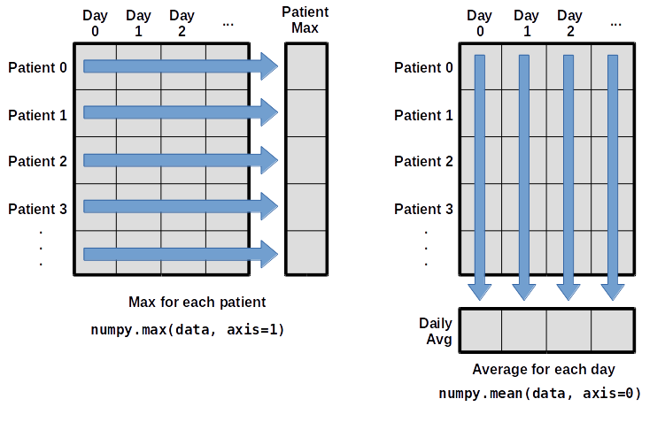
To support this functionality, most array functions allow us to specify the axis we want to work on. If we ask for the average across axis 0 (rows in our 2D example), we get:

print(numpy.mean(data, axis=0))

[  0.           0.45         1.11666667   1.75         2.43333333   3.15
   3.8          3.88333333   5.23333333   5.51666667   5.95         5.9
   8.35         7.73333333   8.36666667   9.5          9.58333333
  10.63333333  11.56666667  12.35        13.25        11.96666667
  11.03333333  10.16666667  10.           8.66666667   9.15         7.25
   7.33333333   6.58333333   6.06666667   5.95         5.11666667   3.6
   3.3          3.56666667   2.48333333   1.5          1.13333333
   0.56666667]

As a quick check, we can ask this array what its shape is:

print(numpy.mean(data, axis=0).shape)

(40,)

The expression (40,) tells us we have an N×1 vector, so this is the average inflammation per day for all patients. If we average across axis 1 (columns in our 2D example), we get:

print(numpy.mean(data, axis=1))

[ 5.45   5.425  6.1    5.9    5.55   6.225  5.975  6.65   6.625  6.525
  6.775  5.8    6.225  5.75   5.225  6.3    6.55   5.7    5.85   6.55
  5.775  5.825  6.175  6.1    5.8    6.425  6.05   6.025  6.175  6.55
  6.175  6.35   6.725  6.125  7.075  5.725  5.925  6.15   6.075  5.75
  5.975  5.725  6.3    5.9    6.75   5.925  7.225  6.15   5.95   6.275  5.7
  6.1    6.825  5.975  6.725  5.7    6.25   6.4    7.05   5.9  ]

which is the average inflammation per patient across all days.

Slicing Strings

A section of an array is called a slice. We can take slices of character strings as well:

element = 'oxygen'
print('first three characters:', element[0:3])
print('last three characters:', element[3:6])

first three characters: oxy
last three characters: gen

What is the value of element[:4]? What about element[4:]? Or element[:]?

Solution

oxyg
en
oxygen

What is element[-1]? What is element[-2]?

Solution

n
e

Given those answers, explain what element[1:-1] does.

Solution

Creates a substring from index 1 up to (not including) the final index, effectively removing the first and last letters from ‘oxygen’

How can we rewrite the slice for getting the last three characters of element, so that it works even if we assign a different string to element? Test your solution with the following strings: carpentry, clone, hi.

Solution

element = 'oxygen'
print('last three characters:', element[-3:])
element = 'carpentry'
print('last three characters:', element[-3:])
element = 'clone'
print('last three characters:', element[-3:])
element = 'hi'
print('last three characters:', element[-3:])

last three characters: gen
last three characters: try
last three characters: one
last three characters: hi

Thin Slices

The expression element[3:3] produces an empty string, i.e., a string that contains no characters. If data holds our array of patient data, what does data[3:3, 4:4] produce? What about data[3:3, :]?

Solution

array([], shape=(0, 0), dtype=float64)
array([], shape=(0, 40), dtype=float64)

Stacking Arrays

Arrays can be concatenated and stacked on top of one another, using NumPy’s vstack and hstack functions for vertical and horizontal stacking, respectively.

import numpy

A = numpy.array([[1,2,3], [4,5,6], [7, 8, 9]])
print('A = ')
print(A)

B = numpy.hstack([A, A])
print('B = ')
print(B)

C = numpy.vstack([A, A])
print('C = ')
print(C)

A =
[[1 2 3]
 [4 5 6]
 [7 8 9]]
B =
[[1 2 3 1 2 3]
 [4 5 6 4 5 6]
 [7 8 9 7 8 9]]
C =
[[1 2 3]
 [4 5 6]
 [7 8 9]
 [1 2 3]
 [4 5 6]
 [7 8 9]]

Write some additional code that slices the first and last columns of A, and stacks them into a 3x2 array. Make sure to print the results to verify your solution.

Solution

A ‘gotcha’ with array indexing is that singleton dimensions are dropped by default. That means A[:, 0] is a one dimensional array, which won’t stack as desired. To preserve singleton dimensions, the index itself can be a slice or array. For example, A[:, :1] returns a two dimensional array with one singleton dimension (i.e. a column vector).

D = numpy.hstack((A[:, :1], A[:, -1:]))
print('D = ')
print(D)

D =
[[1 3]
 [4 6]
 [7 9]]

Solution

An alternative way to achieve the same result is to use Numpy’s delete function to remove the second column of A.

D = numpy.delete(A, 1, 1)
print('D = ')
print(D)

D =
[[1 3]
 [4 6]
 [7 9]]

Change In Inflammation

The patient data is longitudinal in the sense that each row represents a series of observations relating to one individual. This means that the change in inflammation over time is a meaningful concept. Let’s find out how to calculate changes in the data contained in an array with NumPy.

The numpy.diff() function takes an array and returns the differences between two successive values. Let’s use it to examine the changes each day across the first week of patient 3 from our inflammation dataset.

patient3_week1 = data[3, :7]
print(patient3_week1)

 [0. 0. 2. 0. 4. 2. 2.]

Calling numpy.diff(patient3_week1) would do the following calculations

[ 0 - 0, 2 - 0, 0 - 2, 4 - 0, 2 - 4, 2 - 2 ]

and return the 6 difference values in a new array.

numpy.diff(patient3_week1)

array([ 0.,  2., -2.,  4., -2.,  0.])

Note that the array of differences is shorter by one element (length 6).

When calling numpy.diff with a multi-dimensional array, an axis argument may be passed to the function to specify which axis to process. When applying numpy.diff to our 2D inflammation array data, which axis would we specify?

Solution

Since the row axis (0) is patients, it does not make sense to get the difference between two arbitrary patients. The column axis (1) is in days, so the difference is the change in inflammation – a meaningful concept.

numpy.diff(data, axis=1)

If the shape of an individual data file is (60, 40) (60 rows and 40 columns), what would the shape of the array be after you run the diff() function and why?

Solution

The shape will be (60, 39) because there is one fewer difference between columns than there are columns in the data.

How would you find the largest change in inflammation for each patient? Does it matter if the change in inflammation is an increase or a decrease?

Solution

By using the numpy.max() function after you apply the numpy.diff() function, you will get the largest difference between days.

numpy.max(numpy.diff(data, axis=1), axis=1)

array([  7.,  12.,  11.,  10.,  11.,  13.,  10.,   8.,  10.,  10.,   7.,
         7.,  13.,   7.,  10.,  10.,   8.,  10.,   9.,  10.,  13.,   7.,
        12.,   9.,  12.,  11.,  10.,  10.,   7.,  10.,  11.,  10.,   8.,
        11.,  12.,  10.,   9.,  10.,  13.,  10.,   7.,   7.,  10.,  13.,
        12.,   8.,   8.,  10.,  10.,   9.,   8.,  13.,  10.,   7.,  10.,
         8.,  12.,  10.,   7.,  12.])

If inflammation values decrease along an axis, then the difference from one element to the next will be negative. If you are interested in the magnitude of the change and not the direction, the numpy.absolute() function will provide that.

Notice the difference if you get the largest absolute difference between readings.

numpy.max(numpy.absolute(numpy.diff(data, axis=1)), axis=1)

array([ 12.,  14.,  11.,  13.,  11.,  13.,  10.,  12.,  10.,  10.,  10.,
        12.,  13.,  10.,  11.,  10.,  12.,  13.,   9.,  10.,  13.,   9.,
        12.,   9.,  12.,  11.,  10.,  13.,   9.,  13.,  11.,  11.,   8.,
        11.,  12.,  13.,   9.,  10.,  13.,  11.,  11.,  13.,  11.,  13.,
        13.,  10.,   9.,  10.,  10.,   9.,   9.,  13.,  10.,   9.,  10.,
        11.,  13.,  10.,  10.,  12.])

Key Points

• Import a library into a program using import libraryname.

• Use the numpy library to work with arrays in Python.

• The expression array.shape gives the shape of an array.

• Use array[x, y] to select a single element from a 2D array.

• Array indices start at 0, not 1.

• Use low:high to specify a slice that includes the indices from low to high-1.

• Use # some kind of explanation to add comments to programs.

• Use numpy.mean(array), numpy.max(array), and numpy.min(array) to calculate simple statistics.

• Use numpy.mean(array, axis=0) or numpy.mean(array, axis=1) to calculate statistics across the specified axis.

Visualizing Tabular Data

Overview

Teaching: 30 min
Exercises: 20 min

Questions

• How can I visualize tabular data in Python?

• How can I group several plots together?

Objectives

• Plot simple graphs from data.

• Group several graphs in a single figure.

Visualizing data

The mathematician Richard Hamming once said, “The purpose of computing is insight, not numbers,” and the best way to develop insight is often to visualize data. Visualization deserves an entire lecture of its own, but we can explore a few features of Python’s matplotlib library here. While there is no official plotting library, matplotlib is the de facto standard. First, we will import the pyplot module from matplotlib and use two of its functions to create and display a heat map of our data:

import matplotlib.pyplot
image = matplotlib.pyplot.imshow(data)
matplotlib.pyplot.show()

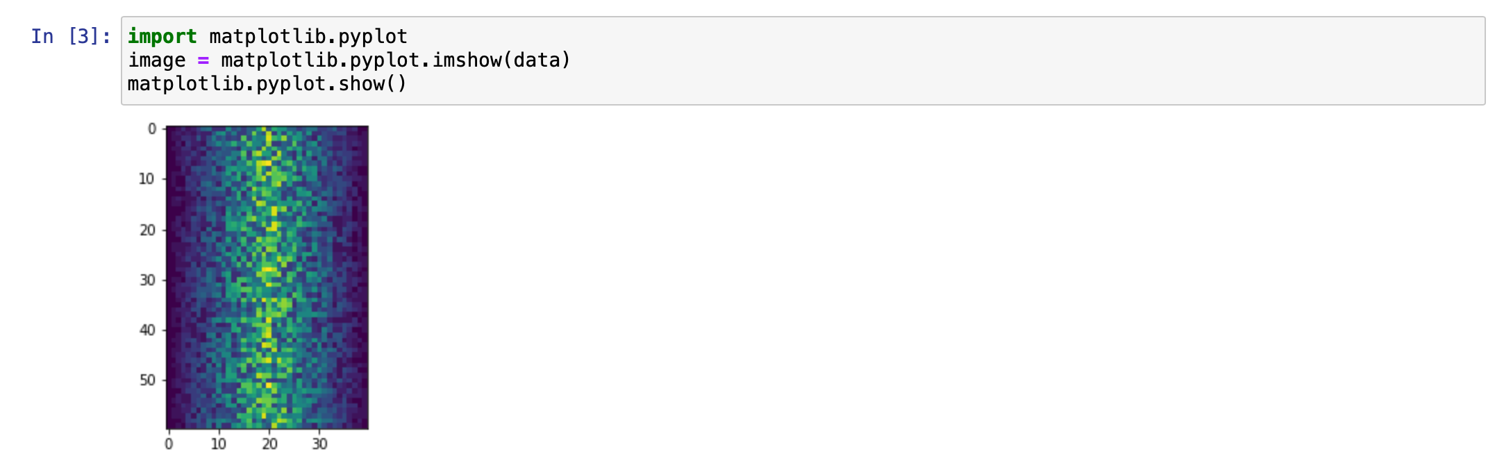
Blue pixels in this heat map represent low values, while yellow pixels represent high values. As we can see, inflammation rises and falls over a 40-day period. Let’s take a look at the average inflammation over time:

ave_inflammation = numpy.mean(data, axis=0)
ave_plot = matplotlib.pyplot.plot(ave_inflammation)
matplotlib.pyplot.show()

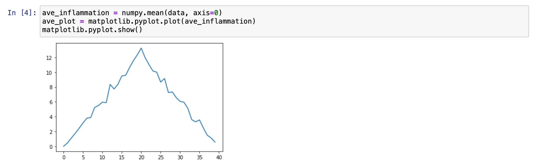
Here, we have put the average inflammation per day across all patients in the variable ave_inflammation, then asked matplotlib.pyplot to create and display a line graph of those values. The result is a roughly linear rise and fall, which is suspicious: we might instead expect a sharper rise and slower fall. Let’s have a look at two other statistics:

max_plot = matplotlib.pyplot.plot(numpy.max(data, axis=0))
matplotlib.pyplot.show()

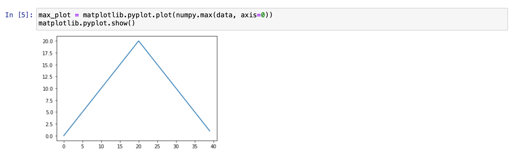
min_plot = matplotlib.pyplot.plot(numpy.min(data, axis=0))
matplotlib.pyplot.show()

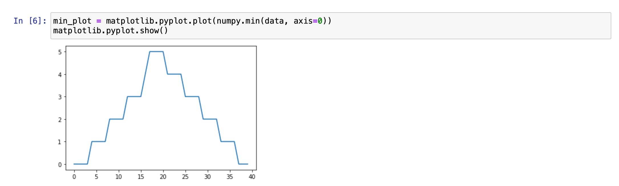
The maximum value rises and falls smoothly, while the minimum seems to be a step function. Neither trend seems particularly likely, so either there’s a mistake in our calculations or something is wrong with our data. This insight would have been difficult to reach by examining the numbers themselves without visualization tools.

Grouping plots

You can group similar plots in a single figure using subplots. This script below uses a number of new commands. The function matplotlib.pyplot.figure() creates a space into which we will place all of our plots. The parameter figsize tells Python how big to make this space. Each subplot is placed into the figure using its add_subplot method. The add_subplot method takes 3 parameters. The first denotes how many total rows of subplots there are, the second parameter refers to the total number of subplot columns, and the final parameter denotes which subplot your variable is referencing (left-to-right, top-to-bottom). Each subplot is stored in a different variable (axes1, axes2, axes3). Once a subplot is created, the axes can be titled using the set_xlabel() command (or set_ylabel()). 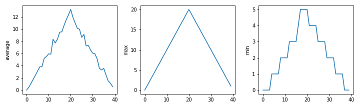Here are our three plots side by side:

import numpy
import matplotlib.pyplot

data = numpy.loadtxt(fname='inflammation-01.csv', delimiter=',')

fig = matplotlib.pyplot.figure(figsize=(10.0, 3.0))

axes1 = fig.add_subplot(1, 3, 1)
axes2 = fig.add_subplot(1, 3, 2)
axes3 = fig.add_subplot(1, 3, 3)

axes1.set_ylabel('average')
axes1.plot(numpy.mean(data, axis=0))

axes2.set_ylabel('max')
axes2.plot(numpy.max(data, axis=0))

axes3.set_ylabel('min')
axes3.plot(numpy.min(data, axis=0))

fig.tight_layout()

matplotlib.pyplot.savefig('inflammation.png')
matplotlib.pyplot.show()

The call to loadtxt reads our data, and the rest of the program tells the plotting library how large we want the figure to be, that we’re creating three subplots, what to draw for each one, and that we want a tight layout. (If we leave out that call to fig.tight_layout(), the graphs will actually be squeezed together more closely.)

The call to savefig stores the plot as a graphics file. This can be a convenient way to store your plots for use in other documents, web pages etc. The graphics format is automatically determined by Matplotlib from the file name ending we specify; here PNG from ‘inflammation.png’. Matplotlib supports many different graphics formats, including SVG, PDF, and JPEG.

Importing libraries with shortcuts

In this lesson we use the import matplotlib.pyplot syntax to import the pyplot module of matplotlib. However, shortcuts such as import matplotlib.pyplot as plt are frequently used. Importing pyplot this way means that after the initial import, rather than writing matplotlib.pyplot.plot(...), you can now write plt.plot(...). Another common convention is to use the shortcut import numpy as np when importing the NumPy library. We then can write np.loadtxt(...) instead of numpy.loadtxt(...), for example.

Some people prefer these shortcuts as it is quicker to type and results in shorter lines of code - especially for libraries with long names! You will frequently see Python code online using a pyplot function with plt, or a NumPy function with np, and it’s because they’ve used this shortcut. It makes no difference which approach you choose to take, but you must be consistent as if you use import matplotlib.pyplot as plt then matplotlib.pyplot.plot(...) will not work, and you must use plt.plot(...) instead. Because of this, when working with other people it is important you agree on how libraries are imported.

Plot Scaling

Why do all of our plots stop just short of the upper end of our graph?

Solution

Because matplotlib normally sets x and y axes limits to the min and max of our data (depending on data range)

If we want to change this, we can use the set_ylim(min, max) method of each ‘axes’, for example:

axes3.set_ylim(0,6)

Update your plotting code to automatically set a more appropriate scale. (Hint: you can make use of the max and min methods to help.)

Solution

# One method
axes3.set_ylabel('min')
axes3.plot(numpy.min(data, axis=0))
axes3.set_ylim(0,6)

Solution

# A more automated approach
min_data = numpy.min(data, axis=0)
axes3.set_ylabel('min')
axes3.plot(min_data)
axes3.set_ylim(numpy.min(min_data), numpy.max(min_data) * 1.1)

Drawing Straight Lines

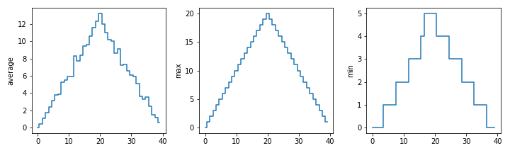
In the center and right subplots above, we expect all lines to look like step functions because non-integer value are not realistic for the minimum and maximum values. However, you can see that the lines are not always vertical or horizontal, and in particular the step function in the subplot on the right looks slanted. Why is this?

Solution

Because matplotlib interpolates (draws a straight line) between the points. One way to do avoid this is to use the Matplotlib drawstyle option:

import numpy
import matplotlib.pyplot

data = numpy.loadtxt(fname='inflammation-01.csv', delimiter=',')

fig = matplotlib.pyplot.figure(figsize=(10.0, 3.0))

axes1 = fig.add_subplot(1, 3, 1)
axes2 = fig.add_subplot(1, 3, 2)
axes3 = fig.add_subplot(1, 3, 3)

axes1.set_ylabel('average')
axes1.plot(numpy.mean(data, axis=0), drawstyle='steps-mid')

axes2.set_ylabel('max')
axes2.plot(numpy.max(data, axis=0), drawstyle='steps-mid')

axes3.set_ylabel('min')
axes3.plot(numpy.min(data, axis=0), drawstyle='steps-mid')

fig.tight_layout()

matplotlib.pyplot.show()

Make Your Own Plot

Create a plot showing the standard deviation (numpy.std) of the inflammation data for each day across all patients.

Solution

std_plot = matplotlib.pyplot.plot(numpy.std(data, axis=0))
matplotlib.pyplot.show()

Moving Plots Around

Modify the program to display the three plots on top of one another instead of side by side.

Solution

import numpy
import matplotlib.pyplot

data = numpy.loadtxt(fname='inflammation-01.csv', delimiter=',')

# change figsize (swap width and height)
fig = matplotlib.pyplot.figure(figsize=(3.0, 10.0))

# change add_subplot (swap first two parameters)
axes1 = fig.add_subplot(3, 1, 1)
axes2 = fig.add_subplot(3, 1, 2)
axes3 = fig.add_subplot(3, 1, 3)

axes1.set_ylabel('average')
axes1.plot(numpy.mean(data, axis=0))

axes2.set_ylabel('max')
axes2.plot(numpy.max(data, axis=0))

axes3.set_ylabel('min')
axes3.plot(numpy.min(data, axis=0))

fig.tight_layout()

matplotlib.pyplot.show()

Key Points

• Use the pyplot module from the matplotlib library for creating simple visualizations.

Reading Tabular Data into DataFrames

Overview

Teaching: 10 min
Exercises: 10 min

Questions

• How can I read tabular data?

Objectives

• Import the Pandas library.

• Use Pandas to load a simple CSV data set.

• Get some basic information about a Pandas DataFrame.

Use the Pandas library to do statistics on tabular data.

• Pandas is a widely-used Python library for statistics, particularly on tabular data.
• Borrows many features from R’s dataframes.
  • A 2-dimensional table whose columns have names and potentially have different data types.
• Load it with import pandas as pd. The alias pd is commonly used for Pandas.
• Read a Comma Separated Values (CSV) data file with pd.read_csv.
  • Argument is the name of the file to be read.
  • Assign result to a variable to store the data that was read.

import pandas as pd

data = pd.read_csv('data/gapminder_gdp_oceania.csv')
print(data)

       country  gdpPercap_1952  gdpPercap_1957  gdpPercap_1962  \
0    Australia     10039.59564     10949.64959     12217.22686
1  New Zealand     10556.57566     12247.39532     13175.67800

   gdpPercap_1967  gdpPercap_1972  gdpPercap_1977  gdpPercap_1982  \
0     14526.12465     16788.62948     18334.19751     19477.00928
1     14463.91893     16046.03728     16233.71770     17632.41040

   gdpPercap_1987  gdpPercap_1992  gdpPercap_1997  gdpPercap_2002  \
0     21888.88903     23424.76683     26997.93657     30687.75473
1     19007.19129     18363.32494     21050.41377     23189.80135

   gdpPercap_2007
0     34435.36744
1     25185.00911

• The columns in a dataframe are the observed variables, and the rows are the observations.
• Pandas uses backslash \ to show wrapped lines when output is too wide to fit the screen.

File Not Found

Our lessons store their data files in a data sub-directory, which is why the path to the file is data/gapminder_gdp_oceania.csv. If you forget to include data/, or if you include it but your copy of the file is somewhere else, you will get a runtime error that ends with a line like this:

FileNotFoundError: [Errno 2] No such file or directory: 'data/gapminder_gdp_oceania.csv'

Use index_col to specify that a column’s values should be used as row headings.

• Row headings are numbers (0 and 1 in this case).
• Really want to index by country.
• Pass the name of the column to read_csv as its index_col parameter to do this.

data = pd.read_csv('data/gapminder_gdp_oceania.csv', index_col='country')
print(data)

             gdpPercap_1952  gdpPercap_1957  gdpPercap_1962  gdpPercap_1967  \
country
Australia       10039.59564     10949.64959     12217.22686     14526.12465
New Zealand     10556.57566     12247.39532     13175.67800     14463.91893

             gdpPercap_1972  gdpPercap_1977  gdpPercap_1982  gdpPercap_1987  \
country
Australia       16788.62948     18334.19751     19477.00928     21888.88903
New Zealand     16046.03728     16233.71770     17632.41040     19007.19129

             gdpPercap_1992  gdpPercap_1997  gdpPercap_2002  gdpPercap_2007
country
Australia       23424.76683     26997.93657     30687.75473     34435.36744
New Zealand     18363.32494     21050.41377     23189.80135     25185.00911

Use the DataFrame.info() method to find out more about a dataframe.

data.info()

<class 'pandas.core.frame.DataFrame'>
Index: 2 entries, Australia to New Zealand
Data columns (total 12 columns):
gdpPercap_1952    2 non-null float64
gdpPercap_1957    2 non-null float64
gdpPercap_1962    2 non-null float64
gdpPercap_1967    2 non-null float64
gdpPercap_1972    2 non-null float64
gdpPercap_1977    2 non-null float64
gdpPercap_1982    2 non-null float64
gdpPercap_1987    2 non-null float64
gdpPercap_1992    2 non-null float64
gdpPercap_1997    2 non-null float64
gdpPercap_2002    2 non-null float64
gdpPercap_2007    2 non-null float64
dtypes: float64(12)
memory usage: 208.0+ bytes

• This is a DataFrame
• Two rows named 'Australia' and 'New Zealand'
• Twelve columns, each of which has two actual 64-bit floating point values.
  • We will talk later about null values, which are used to represent missing observations.
• Uses 208 bytes of memory.

The DataFrame.columns variable stores information about the dataframe’s columns.

• Note that this is data, not a method. (It doesn’t have parentheses.)
  • Like math.pi.
  • So do not use () to try to call it.
• Called a member variable, or just member.

print(data.columns)

Index(['gdpPercap_1952', 'gdpPercap_1957', 'gdpPercap_1962', 'gdpPercap_1967',
       'gdpPercap_1972', 'gdpPercap_1977', 'gdpPercap_1982', 'gdpPercap_1987',
       'gdpPercap_1992', 'gdpPercap_1997', 'gdpPercap_2002', 'gdpPercap_2007'],
      dtype='object')

Use DataFrame.T to transpose a dataframe.

• Sometimes want to treat columns as rows and vice versa.
• Transpose (written .T) doesn’t copy the data, just changes the program’s view of it.
• Like columns, it is a member variable.

print(data.T)

country           Australia  New Zealand
gdpPercap_1952  10039.59564  10556.57566
gdpPercap_1957  10949.64959  12247.39532
gdpPercap_1962  12217.22686  13175.67800
gdpPercap_1967  14526.12465  14463.91893
gdpPercap_1972  16788.62948  16046.03728
gdpPercap_1977  18334.19751  16233.71770
gdpPercap_1982  19477.00928  17632.41040
gdpPercap_1987  21888.88903  19007.19129
gdpPercap_1992  23424.76683  18363.32494
gdpPercap_1997  26997.93657  21050.41377
gdpPercap_2002  30687.75473  23189.80135
gdpPercap_2007  34435.36744  25185.00911

Use DataFrame.describe() to get summary statistics about data.

DataFrame.describe() gets the summary statistics of only the columns that have numerical data. All other columns are ignored, unless you use the argument include='all'.

print(data.describe())

       gdpPercap_1952  gdpPercap_1957  gdpPercap_1962  gdpPercap_1967  \
count        2.000000        2.000000        2.000000        2.000000
mean     10298.085650    11598.522455    12696.452430    14495.021790
std        365.560078      917.644806      677.727301       43.986086
min      10039.595640    10949.649590    12217.226860    14463.918930
25%      10168.840645    11274.086022    12456.839645    14479.470360
50%      10298.085650    11598.522455    12696.452430    14495.021790
75%      10427.330655    11922.958888    12936.065215    14510.573220
max      10556.575660    12247.395320    13175.678000    14526.124650

       gdpPercap_1972  gdpPercap_1977  gdpPercap_1982  gdpPercap_1987  \
count         2.00000        2.000000        2.000000        2.000000
mean      16417.33338    17283.957605    18554.709840    20448.040160
std         525.09198     1485.263517     1304.328377     2037.668013
min       16046.03728    16233.717700    17632.410400    19007.191290
25%       16231.68533    16758.837652    18093.560120    19727.615725
50%       16417.33338    17283.957605    18554.709840    20448.040160
75%       16602.98143    17809.077557    19015.859560    21168.464595
max       16788.62948    18334.197510    19477.009280    21888.889030

       gdpPercap_1992  gdpPercap_1997  gdpPercap_2002  gdpPercap_2007
count        2.000000        2.000000        2.000000        2.000000
mean     20894.045885    24024.175170    26938.778040    29810.188275
std       3578.979883     4205.533703     5301.853680     6540.991104
min      18363.324940    21050.413770    23189.801350    25185.009110
25%      19628.685413    22537.294470    25064.289695    27497.598692
50%      20894.045885    24024.175170    26938.778040    29810.188275
75%      22159.406358    25511.055870    28813.266385    32122.777857
max      23424.766830    26997.936570    30687.754730    34435.367440

• Not particularly useful with just two records, but very helpful when there are thousands.

Reading Other Data

Read the data in gapminder_gdp_americas.csv (which should be in the same directory as gapminder_gdp_oceania.csv) into a variable called americas and display its summary statistics.

Solution

To read in a CSV, we use pd.read_csv and pass the filename 'data/gapminder_gdp_americas.csv' to it. We also once again pass the column name 'country' to the parameter index_col in order to index by country. The summary statistics can be displayed with the DataFrame.describe() method.

americas = pd.read_csv('data/gapminder_gdp_americas.csv', index_col='country')
americas.describe()

Inspecting Data

After reading the data for the Americas, use help(americas.head) and help(americas.tail) to find out what DataFrame.head and DataFrame.tail do.

1. What method call will display the first three rows of this data?
2. What method call will display the last three columns of this data? (Hint: you may need to change your view of the data.)

Solution

1. We can check out the first five rows of americas by executing americas.head() (allowing us to view the head of the DataFrame). We can specify the number of rows we wish to see by specifying the parameter n in our call to americas.head(). To view the first three rows, execute:

   americas.head(n=3)
   

             continent  gdpPercap_1952  gdpPercap_1957  gdpPercap_1962  \
   country
   Argentina  Americas     5911.315053     6856.856212     7133.166023
   Bolivia    Americas     2677.326347     2127.686326     2180.972546
   Brazil     Americas     2108.944355     2487.365989     3336.585802
   
              gdpPercap_1967  gdpPercap_1972  gdpPercap_1977  gdpPercap_1982  \
   country
   Argentina     8052.953021     9443.038526    10079.026740     8997.897412
   Bolivia       2586.886053     2980.331339     3548.097832     3156.510452
   Brazil        3429.864357     4985.711467     6660.118654     7030.835878
   
              gdpPercap_1987  gdpPercap_1992  gdpPercap_1997  gdpPercap_2002  \
   country
   Argentina     9139.671389     9308.418710    10967.281950     8797.640716
   Bolivia       2753.691490     2961.699694     3326.143191     3413.262690
   Brazil        7807.095818     6950.283021     7957.980824     8131.212843
   
              gdpPercap_2007
   country
   Argentina    12779.379640
   Bolivia       3822.137084
   Brazil        9065.800825
   

2. To check out the last three rows of americas, we would use the command, americas.tail(n=3), analogous to head() used above. However, here we want to look at the last three columns so we need to change our view and then use tail(). To do so, we create a new DataFrame in which rows and columns are switched:

   americas_flipped = americas.T
   

   We can then view the last three columns of americas by viewing the last three rows of americas_flipped:

   americas_flipped.tail(n=3)
   

   country        Argentina  Bolivia   Brazil   Canada    Chile Colombia  \
   gdpPercap_1997   10967.3  3326.14  7957.98  28954.9  10118.1  6117.36
   gdpPercap_2002   8797.64  3413.26  8131.21    33329  10778.8  5755.26
   gdpPercap_2007   12779.4  3822.14   9065.8  36319.2  13171.6  7006.58
   
   country        Costa Rica     Cuba Dominican Republic  Ecuador    ...     \
   gdpPercap_1997    6677.05  5431.99             3614.1  7429.46    ...
   gdpPercap_2002    7723.45  6340.65            4563.81  5773.04    ...
   gdpPercap_2007    9645.06   8948.1            6025.37  6873.26    ...
   
   country          Mexico Nicaragua   Panama Paraguay     Peru Puerto Rico  \
   gdpPercap_1997   9767.3   2253.02  7113.69   4247.4  5838.35     16999.4
   gdpPercap_2002  10742.4   2474.55  7356.03  3783.67  5909.02     18855.6
   gdpPercap_2007  11977.6   2749.32  9809.19  4172.84  7408.91     19328.7
   
   country        Trinidad and Tobago United States  Uruguay Venezuela
   gdpPercap_1997             8792.57       35767.4  9230.24   10165.5
   gdpPercap_2002             11460.6       39097.1     7727   8605.05
   gdpPercap_2007             18008.5       42951.7  10611.5   11415.8
   

   This shows the data that we want, but we may prefer to display three columns instead of three rows, so we can flip it back:

   americas_flipped.tail(n=3).T    
   

   Note: we could have done the above in a single line of code by ‘chaining’ the commands:

   americas.T.tail(n=3).T
   

Reading Files in Other Directories

The data for your current project is stored in a file called microbes.csv, which is located in a folder called field_data. You are doing analysis in a notebook called analysis.ipynb in a sibling folder called thesis:

your_home_directory
+-- field_data/
|   +-- microbes.csv
+-- thesis/
    +-- analysis.ipynb

What value(s) should you pass to read_csv to read microbes.csv in analysis.ipynb?

Solution

We need to specify the path to the file of interest in the call to pd.read_csv. We first need to ‘jump’ out of the folder thesis using ‘../’ and then into the folder field_data using ‘field_data/’. Then we can specify the filename `microbes.csv. The result is as follows:

data_microbes = pd.read_csv('../field_data/microbes.csv')

Writing Data

As well as the read_csv function for reading data from a file, Pandas provides a to_csv function to write dataframes to files. Applying what you’ve learned about reading from files, write one of your dataframes to a file called processed.csv. You can use help to get information on how to use to_csv.

Solution

In order to write the DataFrame americas to a file called processed.csv, execute the following command:

americas.to_csv('processed.csv')

For help on to_csv, you could execute, for example:

help(americas.to_csv)

Note that help(to_csv) throws an error! This is a subtlety and is due to the fact that to_csv is NOT a function in and of itself and the actual call is americas.to_csv.

Key Points

• Use the Pandas library to get basic statistics out of tabular data.

• Use index_col to specify that a column’s values should be used as row headings.

• Use DataFrame.info to find out more about a dataframe.

• The DataFrame.columns variable stores information about the dataframe’s columns.

• Use DataFrame.T to transpose a dataframe.

• Use DataFrame.describe to get summary statistics about data.

Pandas DataFrames

Overview

Teaching: 15 min
Exercises: 15 min

Questions

• How can I do statistical analysis of tabular data?

Objectives

• Select individual values from a Pandas dataframe.

• Select entire rows or entire columns from a dataframe.

• Select a subset of both rows and columns from a dataframe in a single operation.

• Select a subset of a dataframe by a single Boolean criterion.

Note about Pandas DataFrames/Series

A DataFrame is a collection of Series; The DataFrame is the way Pandas represents a table, and Series is the data-structure Pandas use to represent a column.

Pandas is built on top of the Numpy library, which in practice means that most of the methods defined for Numpy Arrays apply to Pandas Series/DataFrames.

What makes Pandas so attractive is the powerful interface to access individual records of the table, proper handling of missing values, and relational-databases operations between DataFrames.

Selecting values

To access a value at the position [i,j] of a DataFrame, we have two options, depending on what is the meaning of i in use. Remember that a DataFrame provides an index as a way to identify the rows of the table; a row, then, has a position inside the table as well as a label, which uniquely identifies its entry in the DataFrame.

Use DataFrame.iloc[..., ...] to select values by their (entry) position

• Can specify location by numerical index analogously to 2D version of character selection in strings.

import pandas as pd
data = pd.read_csv('data/gapminder_gdp_europe.csv', index_col='country')
print(data.iloc[0, 0])

1601.056136

Use DataFrame.loc[..., ...] to select values by their (entry) label.

• Can specify location by row name analogously to 2D version of dictionary keys.

print(data.loc["Albania", "gdpPercap_1952"])

1601.056136

Use : on its own to mean all columns or all rows.

• Just like Python’s usual slicing notation.

print(data.loc["Albania", :])

gdpPercap_1952    1601.056136
gdpPercap_1957    1942.284244
gdpPercap_1962    2312.888958
gdpPercap_1967    2760.196931
gdpPercap_1972    3313.422188
gdpPercap_1977    3533.003910
gdpPercap_1982    3630.880722
gdpPercap_1987    3738.932735
gdpPercap_1992    2497.437901
gdpPercap_1997    3193.054604
gdpPercap_2002    4604.211737
gdpPercap_2007    5937.029526
Name: Albania, dtype: float64

• Would get the same result printing data.loc["Albania"] (without a second index).

print(data.loc[:, "gdpPercap_1952"])

country
Albania                    1601.056136
Austria                    6137.076492
Belgium                    8343.105127
⋮ ⋮ ⋮
Switzerland               14734.232750
Turkey                     1969.100980
United Kingdom             9979.508487
Name: gdpPercap_1952, dtype: float64

• Would get the same result printing data["gdpPercap_1952"]
• Also get the same result printing data.gdpPercap_1952 (not recommended, because easily confused with . notation for methods)

Select multiple columns or rows using DataFrame.loc and a named slice.

print(data.loc['Italy':'Poland', 'gdpPercap_1962':'gdpPercap_1972'])

             gdpPercap_1962  gdpPercap_1967  gdpPercap_1972
country
Italy           8243.582340    10022.401310    12269.273780
Montenegro      4649.593785     5907.850937     7778.414017
Netherlands    12790.849560    15363.251360    18794.745670
Norway         13450.401510    16361.876470    18965.055510
Poland          5338.752143     6557.152776     8006.506993

In the above code, we discover that slicing using loc is inclusive at both ends, which differs from slicing using iloc, where slicing indicates everything up to but not including the final index.

Result of slicing can be used in further operations.

• Usually don’t just print a slice.
• All the statistical operators that work on entire dataframes work the same way on slices.
• E.g., calculate max of a slice.

print(data.loc['Italy':'Poland', 'gdpPercap_1962':'gdpPercap_1972'].max())

gdpPercap_1962    13450.40151
gdpPercap_1967    16361.87647
gdpPercap_1972    18965.05551
dtype: float64

print(data.loc['Italy':'Poland', 'gdpPercap_1962':'gdpPercap_1972'].min())

gdpPercap_1962    4649.593785
gdpPercap_1967    5907.850937
gdpPercap_1972    7778.414017
dtype: float64

Use comparisons to select data based on value.

• Comparison is applied element by element.
• Returns a similarly-shaped dataframe of True and False.

# Use a subset of data to keep output readable.
subset = data.loc['Italy':'Poland', 'gdpPercap_1962':'gdpPercap_1972']
print('Subset of data:\n', subset)

# Which values were greater than 10000 ?
print('\nWhere are values large?\n', subset > 10000)

Subset of data:
             gdpPercap_1962  gdpPercap_1967  gdpPercap_1972
country
Italy           8243.582340    10022.401310    12269.273780
Montenegro      4649.593785     5907.850937     7778.414017
Netherlands    12790.849560    15363.251360    18794.745670
Norway         13450.401510    16361.876470    18965.055510
Poland          5338.752143     6557.152776     8006.506993

Where are values large?
            gdpPercap_1962 gdpPercap_1967 gdpPercap_1972
country
Italy                False           True           True
Montenegro           False          False          False
Netherlands           True           True           True
Norway                True           True           True
Poland               False          False          False

Select values or NaN using a Boolean mask.

• A frame full of Booleans is sometimes called a mask because of how it can be used.

mask = subset > 10000
print(subset[mask])

             gdpPercap_1962  gdpPercap_1967  gdpPercap_1972
country
Italy                   NaN     10022.40131     12269.27378
Montenegro              NaN             NaN             NaN
Netherlands     12790.84956     15363.25136     18794.74567
Norway          13450.40151     16361.87647     18965.05551
Poland                  NaN             NaN             NaN

• Get the value where the mask is true, and NaN (Not a Number) where it is false.
• Useful because NaNs are ignored by operations like max, min, average, etc.

print(subset[subset > 10000].describe())

       gdpPercap_1962  gdpPercap_1967  gdpPercap_1972
count        2.000000        3.000000        3.000000
mean     13120.625535    13915.843047    16676.358320
std        466.373656     3408.589070     3817.597015
min      12790.849560    10022.401310    12269.273780
25%      12955.737547    12692.826335    15532.009725
50%      13120.625535    15363.251360    18794.745670
75%      13285.513523    15862.563915    18879.900590
max      13450.401510    16361.876470    18965.055510

Group By: split-apply-combine

Pandas vectorizing methods and grouping operations are features that provide users much flexibility to analyse their data.

For instance, let’s say we want to have a clearer view on how the European countries split themselves according to their GDP.

1. We may have a glance by splitting the countries in two groups during the years surveyed, those who presented a GDP higher than the European average and those with a lower GDP.
2. We then estimate a wealthy score based on the historical (from 1962 to 2007) values, where we account how many times a country has participated in the groups of lower or higher GDP

mask_higher = data > data.mean()
wealth_score = mask_higher.aggregate('sum', axis=1) / len(data.columns)
wealth_score

country
Albania                   0.000000
Austria                   1.000000
Belgium                   1.000000
Bosnia and Herzegovina    0.000000
Bulgaria                  0.000000
Croatia                   0.000000
Czech Republic            0.500000
Denmark                   1.000000
Finland                   1.000000
France                    1.000000
Germany                   1.000000
Greece                    0.333333
Hungary                   0.000000
Iceland                   1.000000
Ireland                   0.333333
Italy                     0.500000
Montenegro                0.000000
Netherlands               1.000000
Norway                    1.000000
Poland                    0.000000
Portugal                  0.000000
Romania                   0.000000
Serbia                    0.000000
Slovak Republic           0.000000
Slovenia                  0.333333
Spain                     0.333333
Sweden                    1.000000
Switzerland               1.000000
Turkey                    0.000000
United Kingdom            1.000000
dtype: float64

Finally, for each group in the wealth_score table, we sum their (financial) contribution across the years surveyed using chained methods:

data.groupby(wealth_score).sum()

          gdpPercap_1952  gdpPercap_1957  gdpPercap_1962  gdpPercap_1967  \
0.000000    36916.854200    46110.918793    56850.065437    71324.848786   
0.333333    16790.046878    20942.456800    25744.935321    33567.667670   
0.500000    11807.544405    14505.000150    18380.449470    21421.846200   
1.000000   104317.277560   127332.008735   149989.154201   178000.350040   

          gdpPercap_1972  gdpPercap_1977  gdpPercap_1982  gdpPercap_1987  \
0.000000    88569.346898   104459.358438   113553.768507   119649.599409   
0.333333    45277.839976    53860.456750    59679.634020    64436.912960   
0.500000    25377.727380    29056.145370    31914.712050    35517.678220   
1.000000   215162.343140   241143.412730   263388.781960   296825.131210   

          gdpPercap_1992  gdpPercap_1997  gdpPercap_2002  gdpPercap_2007  
0.000000    92380.047256   103772.937598   118590.929863   149577.357928  
0.333333    67918.093220    80876.051580   102086.795210   122803.729520  
0.500000    36310.666080    40723.538700    45564.308390    51403.028210  
1.000000   315238.235970   346930.926170   385109.939210   427850.333420

Selection of Individual Values

Assume Pandas has been imported into your notebook and the Gapminder GDP data for Europe has been loaded:

import pandas as pd

df = pd.read_csv('data/gapminder_gdp_europe.csv', index_col='country')

Write an expression to find the Per Capita GDP of Serbia in 2007.

Solution

The selection can be done by using the labels for both the row (“Serbia”) and the column (“gdpPercap_2007”):

print(df.loc['Serbia', 'gdpPercap_2007'])

The output is

9786.534714

Extent of Slicing

1. Do the two statements below produce the same output?
2. Based on this, what rule governs what is included (or not) in numerical slices and named slices in Pandas?

print(df.iloc[0:2, 0:2])
print(df.loc['Albania':'Belgium', 'gdpPercap_1952':'gdpPercap_1962'])

Solution

No, they do not produce the same output! The output of the first statement is:

        gdpPercap_1952  gdpPercap_1957
country                                
Albania     1601.056136     1942.284244
Austria     6137.076492     8842.598030

The second statement gives:

        gdpPercap_1952  gdpPercap_1957  gdpPercap_1962
country                                                
Albania     1601.056136     1942.284244     2312.888958
Austria     6137.076492     8842.598030    10750.721110
Belgium     8343.105127     9714.960623    10991.206760

Clearly, the second statement produces an additional column and an additional row compared to the first statement.
What conclusion can we draw? We see that a numerical slice, 0:2, omits the final index (i.e. index 2) in the range provided, while a named slice, ‘gdpPercap_1952’:’gdpPercap_1962’, includes the final element.

Reconstructing Data

Explain what each line in the following short program does: what is in first, second, etc.?

first = pd.read_csv('data/gapminder_all.csv', index_col='country')
second = first[first['continent'] == 'Americas']
third = second.drop('Puerto Rico')
fourth = third.drop('continent', axis = 1)
fourth.to_csv('result.csv')

Solution

Let’s go through this piece of code line by line.

first = pd.read_csv('data/gapminder_all.csv', index_col='country')

This line loads the dataset containing the GDP data from all countries into a dataframe called first. The index_col='country' parameter selects which column to use as the row labels in the dataframe.

second = first[first['continent'] == 'Americas']

This line makes a selection: only those rows of first for which the ‘continent’ column matches ‘Americas’ are extracted. Notice how the Boolean expression inside the brackets, first['continent'] == 'Americas', is used to select only those rows where the expression is true. Try printing this expression! Can you print also its individual True/False elements? (hint: first assign the expression to a variable)

third = second.drop('Puerto Rico')

As the syntax suggests, this line drops the row from second where the label is ‘Puerto Rico’. The resulting dataframe third has one row less than the original dataframe second.

fourth = third.drop('continent', axis = 1)

Again we apply the drop function, but in this case we are dropping not a row but a whole column. To accomplish this, we need to specify also the axis parameter (we want to drop the second column which has index 1).

fourth.to_csv('result.csv')

The final step is to write the data that we have been working on to a csv file. Pandas makes this easy with the to_csv() function. The only required argument to the function is the filename. Note that the file will be written in the directory from which you started the Jupyter or Python session.

Selecting Indices

Explain in simple terms what idxmin and idxmax do in the short program below. When would you use these methods?

data = pd.read_csv('data/gapminder_gdp_europe.csv', index_col='country')
print(data.idxmin())
print(data.idxmax())

Solution

For each column in data, idxmin will return the index value corresponding to each column’s minimum; idxmax will do accordingly the same for each column’s maximum value.

You can use these functions whenever you want to get the row index of the minimum/maximum value and not the actual minimum/maximum value.

Practice with Selection

Assume Pandas has been imported and the Gapminder GDP data for Europe has been loaded. Write an expression to select each of the following:

1. GDP per capita for all countries in 1982.
2. GDP per capita for Denmark for all years.
3. GDP per capita for all countries for years after 1985.
4. GDP per capita for each country in 2007 as a multiple of GDP per capita for that country in 1952.

Solution

1:

data['gdpPercap_1982']

2:

data.loc['Denmark',:]

3:

data.loc[:,'gdpPercap_1985':]

Pandas is smart enough to recognize the number at the end of the column label and does not give you an error, although no column named gdpPercap_1985 actually exists. This is useful if new columns are added to the CSV file later.

4:

data['gdpPercap_2007']/data['gdpPercap_1952']

Exploring available methods using the dir() function

Python includes a dir() function that can be used to display all of the available methods (functions) that are built into a data object. In Episode 4, we used some methods with a string. But we can see many more are available by using dir():

my_string = 'Hello world!'   # creation of a string object 
dir(myString)

This command returns:

['__add__',
...
'__subclasshook__',
'capitalize',
'casefold',
'center',
...
'upper',
'zfill']

You can use help() or Shift+Tab to get more information about what these methods do.

Assume Pandas has been imported and the Gapminder GDP data for Europe has been loaded as data. Then, use dir() to find the function that prints out the median per-capita GDP across all European countries for each year that information is available.

Solution

Among many choices, dir() lists the median() function as a possibility. Thus,

data.median()

Interpretation

Poland’s borders have been stable since 1945, but changed several times in the years before then. How would you handle this if you were creating a table of GDP per capita for Poland for the entire twentieth century?

Key Points

• Use DataFrame.iloc[..., ...] to select values by integer location.

• Use : on its own to mean all columns or all rows.

• Select multiple columns or rows using DataFrame.loc and a named slice.

• Result of slicing can be used in further operations.

• Use comparisons to select data based on value.

• Select values or NaN using a Boolean mask.

Storing Multiple Values in Lists

Overview

Teaching: 30 min
Exercises: 15 min

Questions

• How can I store many values together?

Objectives

• Explain what a list is.

• Create and index lists of simple values.

• Change the values of individual elements

• Append values to an existing list

• Reorder and slice list elements

• Create and manipulate nested lists

In Python, a list is a way to store multiple values together. In this episode, we will learn how to store multiple values in a list as well as how to work with lists.

Python lists

Unlike NumPy arrays, lists are built into the language so we do not have to load a library to use them. We create a list by putting values inside square brackets and separating the values with commas:

odds = [1, 3, 5, 7]
print('odds are:', odds)

odds are: [1, 3, 5, 7]

We can access elements of a list using indices – numbered positions of elements in the list. These positions are numbered starting at 0, so the first element has an index of 0.

print('first element:', odds[0])
print('last element:', odds[3])
print('"-1" element:', odds[-1])

first element: 1
last element: 7
"-1" element: 7

Yes, we can use negative numbers as indices in Python. When we do so, the index -1 gives us the last element in the list, -2 the second to last, and so on. Because of this, odds[3] and odds[-1] point to the same element here.

There is one important difference between lists and strings: we can change the values in a list, but we cannot change individual characters in a string. For example:

names = ['Curie', 'Darwing', 'Turing']  # typo in Darwin's name
print('names is originally:', names)
names[1] = 'Darwin'  # correct the name
print('final value of names:', names)

names is originally: ['Curie', 'Darwing', 'Turing']
final value of names: ['Curie', 'Darwin', 'Turing']

works, but:

name = 'Darwin'
name[0] = 'd'

---------------------------------------------------------------------------
TypeError                                 Traceback (most recent call last)
<ipython-input-8-220df48aeb2e> in <module>()
      1 name = 'Darwin'
----> 2 name[0] = 'd'

TypeError: 'str' object does not support item assignment

does not.

Ch-Ch-Ch-Ch-Changes

Data which can be modified in place is called mutable, while data which cannot be modified is called immutable. Strings and numbers are immutable. This does not mean that variables with string or number values are constants, but when we want to change the value of a string or number variable, we can only replace the old value with a completely new value.

Lists and arrays, on the other hand, are mutable: we can modify them after they have been created. We can change individual elements, append new elements, or reorder the whole list. For some operations, like sorting, we can choose whether to use a function that modifies the data in-place or a function that returns a modified copy and leaves the original unchanged.

Be careful when modifying data in-place. If two variables refer to the same list, and you modify the list value, it will change for both variables!

salsa = ['peppers', 'onions', 'cilantro', 'tomatoes']
my_salsa = salsa        # <-- my_salsa and salsa point to the *same* list data in memory
salsa[0] = 'hot peppers'
print('Ingredients in my salsa:', my_salsa)

Ingredients in my salsa: ['hot peppers', 'onions', 'cilantro', 'tomatoes']

If you want variables with mutable values to be independent, you must make a copy of the value when you assign it.

salsa = ['peppers', 'onions', 'cilantro', 'tomatoes']
my_salsa = list(salsa)        # <-- makes a *copy* of the list
salsa[0] = 'hot peppers'
print('Ingredients in my salsa:', my_salsa)

Ingredients in my salsa: ['peppers', 'onions', 'cilantro', 'tomatoes']

Because of pitfalls like this, code which modifies data in place can be more difficult to understand. However, it is often far more efficient to modify a large data structure in place than to create a modified copy for every small change. You should consider both of these aspects when writing your code.

Nested Lists

Since a list can contain any Python variables, it can even contain other lists.

For example, we could represent the products in the shelves of a small grocery shop:

x = [['pepper', 'zucchini', 'onion'],
     ['cabbage', 'lettuce', 'garlic'],
     ['apple', 'pear', 'banana']]

Here is a visual example of how indexing a list of lists x works:

Using the previously declared list x, these would be the results of the index operations shown in the image:

print([x[0]])

[['pepper', 'zucchini', 'onion']]

print(x[0])

['pepper', 'zucchini', 'onion']

print(x[0][0])

'pepper'

Thanks to Hadley Wickham for the image above.

Heterogeneous Lists

Lists in Python can contain elements of different types. Example:

sample_ages = [10, 12.5, 'Unknown']

There are many ways to change the contents of lists besides assigning new values to individual elements:

odds.append(11)
print('odds after adding a value:', odds)

odds after adding a value: [1, 3, 5, 7, 11]

removed_element = odds.pop(0)
print('odds after removing the first element:', odds)
print('removed_element:', removed_element)

odds after removing the first element: [3, 5, 7, 11]
removed_element: 1

odds.reverse()
print('odds after reversing:', odds)

odds after reversing: [11, 7, 5, 3]

While modifying in place, it is useful to remember that Python treats lists in a slightly counter-intuitive way.

As we saw earlier, when we modified the salsa list item in-place, if we make a list, (attempt to) copy it and then modify this list, we can cause all sorts of trouble. This also applies to modifying the list using the above functions:

odds = [1, 3, 5, 7]
primes = odds
primes.append(2)
print('primes:', primes)
print('odds:', odds)

primes: [1, 3, 5, 7, 2]
odds: [1, 3, 5, 7, 2]

This is because Python stores a list in memory, and then can use multiple names to refer to the same list. If all we want to do is copy a (simple) list, we can again use the list function, so we do not modify a list we did not mean to:

odds = [1, 3, 5, 7]
primes = list(odds)
primes.append(2)
print('primes:', primes)
print('odds:', odds)

primes: [1, 3, 5, 7, 2]
odds: [1, 3, 5, 7]

Subsets of lists and strings can be accessed by specifying ranges of values in brackets, similar to how we accessed ranges of positions in a NumPy array. This is commonly referred to as “slicing” the list/string.

binomial_name = 'Drosophila melanogaster'
group = binomial_name[0:10]
print('group:', group)

species = binomial_name[11:23]
print('species:', species)

chromosomes = ['X', 'Y', '2', '3', '4']
autosomes = chromosomes[2:5]
print('autosomes:', autosomes)

last = chromosomes[-1]
print('last:', last)

group: Drosophila
species: melanogaster
autosomes: ['2', '3', '4']
last: 4

You can also select non-consecutive elements from a list by slicing with a step size, for example

numbers = [1, 2, 3, 4, 5, 6, 7, 8]
odd_numbers = numbers[0:6:2]
print('odd numbers:', odd_numbers)

odd numbers: [1, 3, 5]

In the above example, numbers[0:2:7] tells python to slice the list numbers from element 0 (1) to element 6 (7), exluded with a step of elements.

Slicing From the End

Use slicing to access only the last four characters of a string or entries of a list.

string_for_slicing = 'Observation date: 02-Feb-2013'
list_for_slicing = [['fluorine', 'F'],
                    ['chlorine', 'Cl'],
                    ['bromine', 'Br'],
                    ['iodine', 'I'],
                    ['astatine', 'At']]

'2013'
[['chlorine', 'Cl'], ['bromine', 'Br'], ['iodine', 'I'], ['astatine', 'At']]

Would your solution work regardless of whether you knew beforehand the length of the string or list (e.g. if you wanted to apply the solution to a set of lists of different lengths)? If not, try to change your approach to make it more robust.

Hint: Remember that indices can be negative as well as positive

Solution

Use negative indices to count elements from the end of a container (such as list or string):

string_for_slicing[-4:]
list_for_slicing[-4:]

If you want to take a slice from the beginning of a sequence, you can omit the first index in the range:

date = 'Monday 4 January 2016'
day = date[0:6]
print('Using 0 to begin range:', day)
day = date[:6]
print('Omitting beginning index:', day)

Using 0 to begin range: Monday
Omitting beginning index: Monday

And similarly, you can omit the ending index in the range to take a slice to the very end of the sequence:

months = ['jan', 'feb', 'mar', 'apr', 'may', 'jun', 'jul', 'aug', 'sep', 'oct', 'nov', 'dec']
sond = months[8:12]
print('With known last position:', sond)
sond = months[8:len(months)]
print('Using len() to get last entry:', sond)
sond = months[8:]
print('Omitting ending index:', sond)

With known last position: ['sep', 'oct', 'nov', 'dec']
Using len() to get last entry: ['sep', 'oct', 'nov', 'dec']
Omitting ending index: ['sep', 'oct', 'nov', 'dec']

Overloading

+ usually means addition, but when used on strings or lists, it means “concatenate”. Given that, what do you think the multiplication operator * does on lists? In particular, what will be the output of the following code?

counts = [2, 4, 6, 8, 10]
repeats = counts * 2
print(repeats)

1. [2, 4, 6, 8, 10, 2, 4, 6, 8, 10]
2. [4, 8, 12, 16, 20]
3. [[2, 4, 6, 8, 10],[2, 4, 6, 8, 10]]
4. [2, 4, 6, 8, 10, 4, 8, 12, 16, 20]

The technical term for this is operator overloading: a single operator, like + or *, can do different things depending on what it’s applied to.

Solution

The multiplication operator * used on a list replicates elements of the list and concatenates them together:

[2, 4, 6, 8, 10, 2, 4, 6, 8, 10]

It’s equivalent to:

counts + counts

Key Points

• [value1, value2, value3, ...] creates a list.

• Lists can contain any Python object, including lists (i.e., list of lists).

• Lists are indexed and sliced with square brackets (e.g., list[0] and list[2:9]), in the same way as strings and arrays.

• Lists are mutable (i.e., their values can be changed in place).

• Strings are immutable (i.e., the characters in them cannot be changed).

For Loops

Overview

Teaching: 10 min
Exercises: 15 min

Questions

• How can I make a program do many things?

Objectives

• Explain what for loops are normally used for.

• Trace the execution of a simple (unnested) loop and correctly state the values of variables in each iteration.

• Write for loops that use the Accumulator pattern to aggregate values.

A for loop executes commands once for each value in a collection.

• Doing calculations on the values in a list one by one is as painful as working with pressure_001, pressure_002, etc.
• A for loop tells Python to execute some statements once for each value in a list, a character string, or some other collection.
• “for each thing in this group, do these operations”

for number in [2, 3, 5]:
    print(number)

• This for loop is equivalent to:

print(2)
print(3)
print(5)

• And the for loop’s output is:

2
3
5

A for loop is made up of a collection, a loop variable, and a body.

for number in [2, 3, 5]:
    print(number)

• The collection, [2, 3, 5], is what the loop is being run on.
• The body, print(number), specifies what to do for each value in the collection.
• The loop variable, number, is what changes for each iteration of the loop.
  • The “current thing”.

The first line of the for loop must end with a colon, and the body must be indented.

• The colon at the end of the first line signals the start of a block of statements.
• Python uses indentation rather than {} or begin/end to show nesting.
  • Any consistent indentation is legal, but almost everyone uses four spaces.

for number in [2, 3, 5]:
print(number)

IndentationError: expected an indented block

• Indentation is always meaningful in Python.

firstName = "Jon"
  lastName = "Smith"

  File "<ipython-input-7-f65f2962bf9c>", line 2
    lastName = "Smith"
    ^
IndentationError: unexpected indent

• This error can be fixed by removing the extra spaces at the beginning of the second line.

Loop variables can be called anything.

• As with all variables, loop variables are:
  • Created on demand.
  • Meaningless: their names can be anything at all.

for kitten in [2, 3, 5]:
    print(kitten)

The body of a loop can contain many statements.

• But no loop should be more than a few lines long.
• Hard for human beings to keep larger chunks of code in mind.

primes = [2, 3, 5]
for p in primes:
    squared = p ** 2
    cubed = p ** 3
    print(p, squared, cubed)

2 4 8
3 9 27
5 25 125

Use range to iterate over a sequence of numbers.

• The built-in function range produces a sequence of numbers.
  • Not a list: the numbers are produced on demand to make looping over large ranges more efficient.
• range(N) is the numbers 0..N-1
  • Exactly the legal indices of a list or character string of length N

print('a range is not a list: range(0, 3)')
for number in range(0, 3):
    print(number)

a range is not a list: range(0, 3)
0
1
2

The Accumulator pattern turns many values into one.

• A common pattern in programs is to:
  1. Initialize an accumulator variable to zero, the empty string, or the empty list.
  2. Update the variable with values from a collection.

# Sum the first 10 integers.
total = 0
for number in range(10):
   total = total + (number + 1)
print(total)

55

• Read total = total + (number + 1) as:
  • Add 1 to the current value of the loop variable number.
  • Add that to the current value of the accumulator variable total.
  • Assign that to total, replacing the current value.
• We have to add number + 1 because range produces 0..9, not 1..10.

Classifying Errors

Is an indentation error a syntax error or a runtime error?

Solution

An IndentationError is a syntax error. Programs with syntax errors cannot be started. A program with a runtime error will start but an error will be thrown under certain conditions.

Tracing Execution

Create a table showing the numbers of the lines that are executed when this program runs, and the values of the variables after each line is executed.

total = 0
for char in "tin":
    total = total + 1

Solution

Line no	Variables
1	total = 0
2	total = 0 char = ‘t’
3	total = 1 char = ‘t’
2	total = 1 char = ‘i’
3	total = 2 char = ‘i’
2	total = 2 char = ‘n’
3	total = 3 char = ‘n’

Reversing a String

Fill in the blanks in the program below so that it prints “nit” (the reverse of the original character string “tin”).

original = "tin"
result = ____
for char in original:
    result = ____
print(result)

Solution

original = "tin"
result = ""
for char in original:
    result = char + result
print(result)

Practice Accumulating

Fill in the blanks in each of the programs below to produce the indicated result.

# Total length of the strings in the list: ["red", "green", "blue"] => 12
total = 0
for word in ["red", "green", "blue"]:
    ____ = ____ + len(word)
print(total)

Solution

total = 0
for word in ["red", "green", "blue"]:
    total = total + len(word)
print(total)

# List of word lengths: ["red", "green", "blue"] => [3, 5, 4]
lengths = ____
for word in ["red", "green", "blue"]:
    lengths.____(____)
print(lengths)

Solution

lengths = []
for word in ["red", "green", "blue"]:
    lengths.append(len(word))
print(lengths)

# Concatenate all words: ["red", "green", "blue"] => "redgreenblue"
words = ["red", "green", "blue"]
result = ____
for ____ in ____:
    ____
print(result)

Solution

words = ["red", "green", "blue"]
result = ""
for word in words:
    result = result + word
print(result)

Create an acronym: Starting from the list ["red", "green", "blue"], create the acronym "RGB" using a for loop.

Hint: You may need to use a string method to properly format the acronym.

Solution

acronym = ""
for word in ["red", "green", "blue"]:
    acronym = acronym + word[0].upper()
print(acronym)

Cumulative Sum

Reorder and properly indent the lines of code below so that they print a list with the cumulative sum of data. The result should be [1, 3, 5, 10].

cumulative.append(total)
for number in data:
cumulative = []
total += number
total = 0
print(cumulative)
data = [1,2,2,5]

Solution

total = 0
data = [1,2,2,5]
cumulative = []
for number in data:
    total += number
    cumulative.append(total)
print(cumulative)

Identifying Variable Name Errors

1. Read the code below and try to identify what the errors are without running it.
2. Run the code and read the error message. What type of NameError do you think this is? Is it a string with no quotes, a misspelled variable, or a variable that should have been defined but was not?
3. Fix the error.
4. Repeat steps 2 and 3, until you have fixed all the errors.

for number in range(10):
    # use a if the number is a multiple of 3, otherwise use b
    if (Number % 3) == 0:
        message = message + a
    else:
        message = message + "b"
print(message)

Solution

• Python variable names are case sensitive: number and Number refer to different variables.
• The variable message needs to be initialized as an empty string.
• We want to add the string "a" to message, not the undefined variable a.

message = ""
for number in range(10):
    # use a if the number is a multiple of 3, otherwise use b
    if (number % 3) == 0:
        message = message + "a"
    else:
        message = message + "b"
print(message)

Identifying Item Errors

1. Read the code below and try to identify what the errors are without running it.
2. Run the code, and read the error message. What type of error is it?
3. Fix the error.

seasons = ['Spring', 'Summer', 'Fall', 'Winter']
print('My favorite season is ', seasons[4])

Solution

This list has 4 elements and the index to access the last element in the list is 3.

seasons = ['Spring', 'Summer', 'Fall', 'Winter']
print('My favorite season is ', seasons[3])

Key Points

• A for loop executes commands once for each value in a collection.

• A for loop is made up of a collection, a loop variable, and a body.

• The first line of the for loop must end with a colon, and the body must be indented.

• Indentation is always meaningful in Python.

• Loop variables can be called anything (but it is strongly advised to have a meaningful name to the looping variable).

• The body of a loop can contain many statements.

• Use range to iterate over a sequence of numbers.

• The Accumulator pattern turns many values into one.

Conditionals

Overview

Teaching: 10 min
Exercises: 15 min

Questions

• How can programs do different things for different data?

Objectives

• Correctly write programs that use if and else statements and simple Boolean expressions (without logical operators).

• Trace the execution of unnested conditionals and conditionals inside loops.

Use if statements to control whether or not a block of code is executed.

• An if statement (more properly called a conditional statement) controls whether some block of code is executed or not.
• Structure is similar to a for statement:
  • First line opens with if and ends with a colon
  • Body containing one or more statements is indented (usually by 4 spaces)

mass = 3.54
if mass > 3.0:
    print(mass, 'is large')

mass = 2.07
if mass > 3.0:
    print(mass, 'is large')

3.54 is large

Conditionals are often used inside loops.

• Not much point using a conditional when we know the value (as above).
• But useful when we have a collection to process.

masses = [3.54, 2.07, 9.22, 1.86, 1.71]
for m in masses:
    if m > 3.0:
        print(m, 'is large')

3.54 is large
9.22 is large

Use else to execute a block of code when an if condition is not true.

• else can be used following an if.
• Allows us to specify an alternative to execute when the if branch isn’t taken.

masses = [3.54, 2.07, 9.22, 1.86, 1.71]
for m in masses:
    if m > 3.0:
        print(m, 'is large')
    else:
        print(m, 'is small')

3.54 is large
2.07 is small
9.22 is large
1.86 is small
1.71 is small

Use elif to specify additional tests.

• May want to provide several alternative choices, each with its own test.
• Use elif (short for “else if”) and a condition to specify these.
• Always associated with an if.
• Must come before the else (which is the “catch all”).

masses = [3.54, 2.07, 9.22, 1.86, 1.71]
for m in masses:
    if m > 9.0:
        print(m, 'is HUGE')
    elif m > 3.0:
        print(m, 'is large')
    else:
        print(m, 'is small')

3.54 is large
2.07 is small
9.22 is HUGE
1.86 is small
1.71 is small

Conditions are tested once, in order.

• Python steps through the branches of the conditional in order, testing each in turn.
• So ordering matters.

grade = 85
if grade >= 70:
    print('grade is C')
elif grade >= 80:
    print('grade is B')
elif grade >= 90:
    print('grade is A')

grade is C

• Does not automatically go back and re-evaluate if values change.

velocity = 10.0
if velocity > 20.0:
    print('moving too fast')
else:
    print('adjusting velocity')
    velocity = 50.0

adjusting velocity

• Often use conditionals in a loop to “evolve” the values of variables.

velocity = 10.0
for i in range(5): # execute the loop 5 times
    print(i, ':', velocity)
    if velocity > 20.0:
        print('moving too fast')
        velocity = velocity - 5.0
    else:
        print('moving too slow')
        velocity = velocity + 10.0
print('final velocity:', velocity)

0 : 10.0
moving too slow
1 : 20.0
moving too slow
2 : 30.0
moving too fast
3 : 25.0
moving too fast
4 : 20.0
moving too slow
final velocity: 30.0

Create a table showing variables’ values to trace a program’s execution.

• The program must have a print statement outside the body of the loop to show the final value of velocity, since its value is updated by the last iteration of the loop.

Compound Relations Using and, or, and Parentheses

Often, you want some combination of things to be true. You can combine relations within a conditional using and and or. Continuing the example above, suppose you have

mass     = [ 3.54,  2.07,  9.22,  1.86,  1.71]
velocity = [10.00, 20.00, 30.00, 25.00, 20.00]

i = 0
for i in range(5):
    if mass[i] > 5 and velocity[i] > 20:
        print("Fast heavy object.  Duck!")
    elif mass[i] > 2 and mass[i] <= 5 and velocity[i] <= 20:
        print("Normal traffic")
    elif mass[i] <= 2 and velocity[i] <= 20:
        print("Slow light object.  Ignore it")
    else:
        print("Whoa!  Something is up with the data.  Check it")

Just like with arithmetic, you can and should use parentheses whenever there is possible ambiguity. A good general rule is to always use parentheses when mixing and and or in the same condition. That is, instead of:

if mass[i] <= 2 or mass[i] >= 5 and velocity[i] > 20:

write one of these:

if (mass[i] <= 2 or mass[i] >= 5) and velocity[i] > 20:
if mass[i] <= 2 or (mass[i] >= 5 and velocity[i] > 20):

so it is perfectly clear to a reader (and to Python) what you really mean.